Soft Segmentation Tutorial (Lite version)¶

Here, we provide a lite version of cell segmentation for SMURF using the FFPE Mouse Brain data from 10x. Notably, this version does not require any GPU resources.

Dataset Information¶

Access the dataset here: Visium HD CytAssist Gene Expression Libraries of Mouse Brain

Important Downloads¶

To download the necessary files, run the following commands:

# Download data from 10x
!mkdir -p "smurf_example_data"
!wget -P smurf_example_data https://cf.10xgenomics.com/samples/spatial-exp/3.0.0/Visium_HD_Mouse_Brain/Visium_HD_Mouse_Brain_tissue_image.tif
!wget -P smurf_example_data https://cf.10xgenomics.com/samples/spatial-exp/3.0.0/Visium_HD_Mouse_Brain/Visium_HD_Mouse_Brain_binned_outputs.tar.gz
!tar -xzvf smurf_example_data/Visium_HD_Mouse_Brain_binned_outputs.tar.gz -C smurf_example_data

# Download our nuclei segmentation results if needed
!curl -L -o smurf_example_data/segmentation_final.npy.gz https://github.com/The-Mitra-Lab/SMURF/raw/main/data/segmentation_final.npy.gz
!gunzip smurf_example_data/segmentation_final.npy.gz

If you use the same cell segmentation method as introduced, you may skip the first part until the section labeled Start here.

[1]:

import numpy as np
import pandas as pd
import matplotlib.pyplot as plt

import scanpy as sc
import anndata

import smurf as su

import pickle
import copy
import gzip

Note on software versions

This tutorial was developed and tested with the exact package versions listed below.

Using these versions should reproduce the results exactly.

Newer releases may introduce subtle differences.

If you encounter any issues, please open an issue on our GitHub repository and we’ll respond as soon as possible. Thanks!

Package	Version
numpy	1.26.4
pandas	1.5.3
tqdm	4.66.2
scanpy	1.10.0
scipy	1.12.0
matplotlib	3.8.3
numba	0.59.0
scikit-learn	1.4.1.post1
Pillow	10.2.0
anndata	0.10.6
h5py	3.10.0
pyarrow	16.1.0
igraph	0.11.5

Here are the python codes you can use to install the exact versions:

import importlib.metadata as metadata
import subprocess
import sys

# Dictionary of desired package versions
desired_versions = {
    "numpy": "1.26.4",
    "pandas": "1.5.3",
    "tqdm": "4.66.2",
    "scanpy": "1.10.0",
    "scipy": "1.12.0",
    "matplotlib": "3.8.3",
    "numba": "0.59.0",
    "scikit-learn": "1.4.1.post1",
    "Pillow": "10.2.0",
    "anndata": "0.10.6",
    "h5py": "3.10.0",
    "pyarrow": "16.1.0",
    "igraph": "0.11.5",
}

for pkg, target_ver in desired_versions.items():
    try:
        installed_ver = metadata.version(pkg)
    except metadata.PackageNotFoundError:
        installed_ver = None

    if installed_ver != target_ver:
        print(f"{pkg} current version: {installed_ver or 'not installed'}, installing/upgrading to {target_ver}…")
        subprocess.run(
            [sys.executable, "-m", "pip", "install", f"{pkg}=={target_ver}"],
            check=True
        )
    else:
        print(f"{pkg} is already at version {target_ver}, no action needed.")

Here, we define your data path and saving path. Ensure that your data path includes the complete HE or DAPI image and a folder containing square_002um data. Specifically, you will need tissue_positions.parquet and filtered_feature_bc_matrix.

[2]:

import os

data_path = 'smurf_example_data/'
save_path = 'results_example_mousebrain/'

# Check if the directory exists
if not os.path.exists(save_path):
    # If it doesn't exist, create it
    os.makedirs(save_path)

We start building our So (spatial object). The input should be your tissue_positions.parquet in 'square_002um/spatial', the final full image, and the format of your experiment (either 'HE' or 'DAPI').

[3]:

so = su.prepare_dataframe_image(data_path+'binned_outputs/square_002um/spatial/tissue_positions.parquet',
                                data_path+'Visium_HD_Mouse_Brain_tissue_image.tif',
                               'HE')

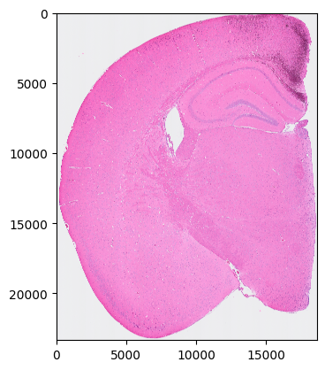
Please use your own tools to perform cell segmentation on so.image_temp() (the area covered by Visium HD in the original image). Set all background pixels to 0 and assign each cell a unique integer cell ID. segmentation_final should be a NumPy array with the same shape as so.image_temp().

[4]:

plt.imshow(so.image_temp())
plt.show()
plt.close()

../../_images/tutorials_notebooks_Tutorial_Mousebrian_8_0.png

Please save the image for segmentation now.

[5]:

with gzip.GzipFile(data_path + 'image_to_segmentation.npy.gz', 'w') as f:
    np.save(f, so.image_temp())

Assuming we now have the final segmentation results, let’s proceed to read them. You can always use the provided example results to try out the tutorial.

[6]:

so.segmentation_final = np.load(data_path + 'segmentation_final.npy')

Now, we start generating cell and spot information to prepare for the analysis.

[7]:

so.generate_cell_spots_information()

Generating cells information.

100%|██████████| 23340/23340 [01:11<00:00, 325.04it/s]

Generating spots information.

100%|██████████| 23340/23340 [02:58<00:00, 130.51it/s]

Filtering cells
We have 57300 nuclei in total.
Creating NN network

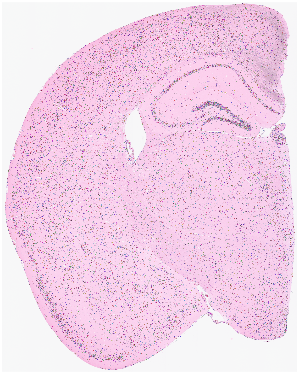
Visualize the nuclei segmentation results overlaid on the original HE or DAPI image. Ensure that the results are meaningful and that the segmented nuclei accurately align with the original image.

[8]:

su.plot_results(so.image_temp(), so.segmentation_final )

../../_images/tutorials_notebooks_Tutorial_Mousebrian_16_0.png

Start Here¶

if you use the same cell segmentation method as introduced:

import numpy as np
import pandas as pd
import matplotlib.pyplot as plt

import scanpy as sc
import anndata

import smurf as su

import pickle
import copy


with open(save_path + 'so.pkl', 'rb') as file:
    so = pickle.load(file)

Load adata from the original the 2um results.

[9]:

# load adata from original 2um results

adata = sc.read_10x_mtx(data_path +'binned_outputs/square_002um/filtered_feature_bc_matrix')
adata = copy.deepcopy(adata[so.df[so.df.in_tissue == 1]['barcode']])
adata.obs

[9]:


s_002um_02448_01644-1
s_002um_00700_02130-1
s_002um_00305_01021-1
s_002um_02703_00756-1
s_002um_02278_00850-1
...
s_002um_02189_01783-1
s_002um_01609_01578-1
s_002um_00456_02202-1
s_002um_00292_01011-1
s_002um_00865_01560-1

6296688 rows × 0 columns

[10]:

sc.pp.filter_genes(adata, min_counts=1000)

Here, we begin by generating the nuclei*genes matrix. The result will be stored in so.final_nuclei.

[11]:

su.nuclei_rna(adata,so)
adata_sc = copy.deepcopy(so.final_nuclei)
adata_sc

100%|██████████| 57300/57300 [01:12<00:00, 795.14it/s]

[11]:

AnnData object with n_obs × n_vars = 57300 × 9970
    var: 'gene_ids', 'feature_types'

Filter cells by counts while preserving the raw data version.

[12]:

sc.pp.filter_cells(adata_sc, min_counts=5)
adata_raw = copy.deepcopy(adata_sc)
adata_raw

[12]:

AnnData object with n_obs × n_vars = 56867 × 9970
    obs: 'n_counts'
    var: 'gene_ids', 'feature_types'

[13]:

adata_raw = copy.deepcopy(adata_sc)

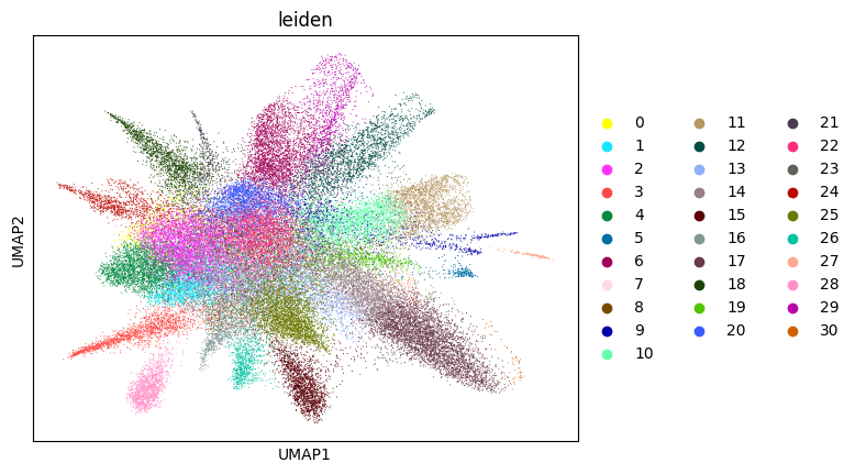
Initial analysis of nuclei data. Note that many datasets may not perform well at this stage; it is normal to observe hundreds of clusters due to low-quality nuclei counts.

[14]:

adata_sc = su.singlecellanalysis(adata_sc,resolution=2)

Starting mt
Starting normalization
Starting PCA
Starting UMAP

/home/juanru/miniconda3/envs/bidcell/lib/python3.10/site-packages/tqdm/auto.py:21: TqdmWarning: IProgress not found. Please update jupyter and ipywidgets. See https://ipywidgets.readthedocs.io/en/stable/user_install.html
  from .autonotebook import tqdm as notebook_tqdm

Starting Clustering

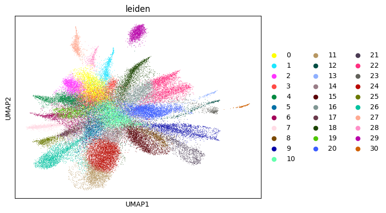
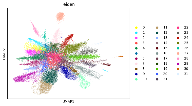
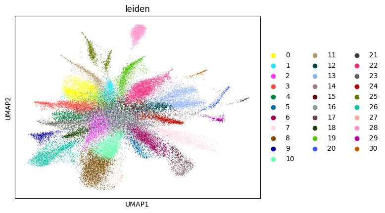
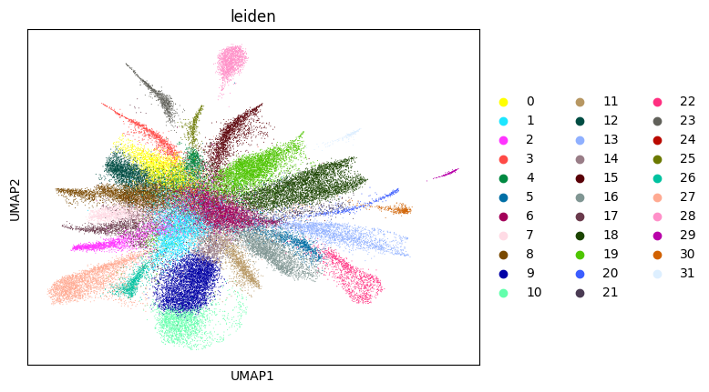
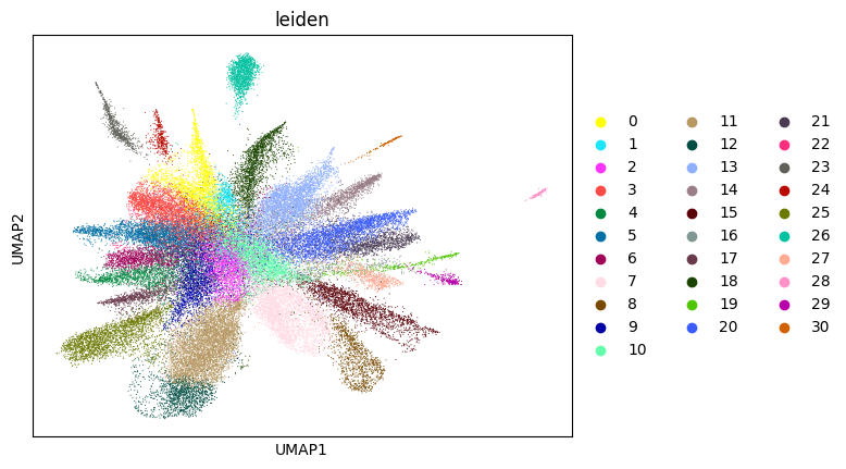
../../_images/tutorials_notebooks_Tutorial_Mousebrian_27_3.png

Here, we start performing iterations. Note that this function can be time-consuming.

[15]:

su.itering_arragement(adata_sc, adata_raw, adata, so, resolution=2, save_folder = save_path, show = True, keep_previous = False)

100%|██████████| 56867/56867 [03:54<00:00, 242.84it/s]
100%|██████████| 56867/56867 [01:07<00:00, 844.55it/s]

Starting mt
Starting normalization
Starting PCA
Starting UMAP
Starting Clustering
WARNING: saving figure to file figures/umap1_umap.png

../../_images/tutorials_notebooks_Tutorial_Mousebrian_29_2.png

0.42855472274655915 1

100%|██████████| 56867/56867 [03:47<00:00, 249.52it/s]
100%|██████████| 56867/56867 [01:04<00:00, 875.60it/s]

Starting mt
Starting normalization
Starting PCA
Starting UMAP
Starting Clustering
WARNING: saving figure to file figures/umap2_umap.png

../../_images/tutorials_notebooks_Tutorial_Mousebrian_29_6.png

0.6737852847699389 2

100%|██████████| 56867/56867 [04:43<00:00, 200.25it/s]
100%|██████████| 56867/56867 [01:04<00:00, 876.07it/s]

Starting mt
Starting normalization
Starting PCA
Starting UMAP
Starting Clustering
WARNING: saving figure to file figures/umap3_umap.png

../../_images/tutorials_notebooks_Tutorial_Mousebrian_29_10.png

0.6851827106003304 3

100%|██████████| 56867/56867 [04:29<00:00, 211.11it/s]
100%|██████████| 56867/56867 [01:05<00:00, 873.54it/s]

Starting mt
Starting normalization
Starting PCA
Starting UMAP
Starting Clustering
WARNING: saving figure to file figures/umap4_umap.png

../../_images/tutorials_notebooks_Tutorial_Mousebrian_29_14.png

0.6991060339712426 4

100%|██████████| 56867/56867 [04:26<00:00, 213.75it/s]
100%|██████████| 56867/56867 [01:05<00:00, 873.39it/s]

Starting mt
Starting normalization
Starting PCA
Starting UMAP
Starting Clustering
WARNING: saving figure to file figures/umap5_umap.png

../../_images/tutorials_notebooks_Tutorial_Mousebrian_29_18.png

0.7115321705141411 5

100%|██████████| 56867/56867 [04:39<00:00, 203.12it/s]
100%|██████████| 56867/56867 [01:05<00:00, 874.69it/s]

Starting mt
Starting normalization
Starting PCA
Starting UMAP
Starting Clustering
WARNING: saving figure to file figures/umap6_umap.png

../../_images/tutorials_notebooks_Tutorial_Mousebrian_29_22.png

0.7026397798438843 6

100%|██████████| 56867/56867 [04:09<00:00, 228.00it/s]
100%|██████████| 56867/56867 [01:05<00:00, 864.88it/s]

Starting mt
Starting normalization
Starting PCA
Starting UMAP
Starting Clustering
WARNING: saving figure to file figures/umap7_umap.png

../../_images/tutorials_notebooks_Tutorial_Mousebrian_29_26.png

0.7168787361641524 7

100%|██████████| 56867/56867 [04:24<00:00, 215.08it/s]
100%|██████████| 56867/56867 [01:05<00:00, 869.83it/s]

Starting mt
Starting normalization
Starting PCA
Starting UMAP
Starting Clustering
WARNING: saving figure to file figures/umap8_umap.png

../../_images/tutorials_notebooks_Tutorial_Mousebrian_29_30.png

0.7257587985649782 8

100%|██████████| 56867/56867 [04:02<00:00, 234.51it/s]
100%|██████████| 56867/56867 [01:05<00:00, 870.64it/s]

Starting mt
Starting normalization
Starting PCA
Starting UMAP
Starting Clustering
WARNING: saving figure to file figures/umap9_umap.png

../../_images/tutorials_notebooks_Tutorial_Mousebrian_29_34.png

0.7143527047493291 9

100%|██████████| 56867/56867 [04:09<00:00, 227.51it/s]
100%|██████████| 56867/56867 [01:05<00:00, 871.23it/s]

Starting mt
Starting normalization
Starting PCA
Starting UMAP
Starting Clustering
WARNING: saving figure to file figures/umap10_umap.png

../../_images/tutorials_notebooks_Tutorial_Mousebrian_29_38.png

0.727594845907013 10

100%|██████████| 56867/56867 [03:55<00:00, 241.17it/s]
100%|██████████| 56867/56867 [01:04<00:00, 875.04it/s]

Starting mt
Starting normalization
Starting PCA
Starting UMAP
Starting Clustering
WARNING: saving figure to file figures/umap11_umap.png

../../_images/tutorials_notebooks_Tutorial_Mousebrian_29_42.png

0.7297884224086874 11

100%|██████████| 56867/56867 [03:59<00:00, 237.50it/s]
100%|██████████| 56867/56867 [01:05<00:00, 872.02it/s]

Starting mt
Starting normalization
Starting PCA
Starting UMAP
Starting Clustering
WARNING: saving figure to file figures/umap12_umap.png

../../_images/tutorials_notebooks_Tutorial_Mousebrian_29_46.png

0.7170889477340182 12

100%|██████████| 56867/56867 [03:53<00:00, 243.56it/s]
100%|██████████| 56867/56867 [01:05<00:00, 873.93it/s]

Starting mt
Starting normalization
Starting PCA
Starting UMAP
Starting Clustering
WARNING: saving figure to file figures/umap13_umap.png

../../_images/tutorials_notebooks_Tutorial_Mousebrian_29_50.png

0.7230415454949939 13

Load results here. Note that the full version differs from the simple version from this point onward. This is your last chance to switch to the full version. (Note that adatas_final, cells_final and weights_record can be used directly there.)

[16]:

adatas_final = sc.read_h5ad(save_path +'adatas.h5ad')

with open(save_path +'cells_final.pkl', 'rb') as file:
    cells_final = pickle.load(file)

with open(save_path +'weights_record.pkl', 'rb') as file:
    weights_record = pickle.load(file)

[17]:

cell_cluster_final = su.return_celltype_plot(adatas_final, so)
su.plot_cellcluster_position(cell_cluster_final, col_num=5)

100%|██████████| 23340/23340 [01:17<00:00, 302.57it/s]

../../_images/tutorials_notebooks_Tutorial_Mousebrian_32_1.png

Here, we generate the final result. By setting plot = True, we will create so.pixels_cells, which might take more than half an hour. If you do not need this or have already generated so.pixels_cells, set plot = False.

Here, adata_sc_final.obs contains five columns:

cell_cluster: Denotes the cluster assignment from the iteration.
cos_simularity: The cosine similarity of the cell’s gene expression with the average expression of its cluster.
cell_size: The number of 2um spots occupied by this cell.
x and y: The absolute coordinates of the cell, matching the spot locations provided by 10x.

[18]:

adata_sc_final = su.get_finaldata_fast(cells_final, so, adatas_final, adata, weights_record, plot = True)
adata_sc_final

100%|██████████| 1638546/1638546 [01:29<00:00, 18378.01it/s]
100%|██████████| 23340/23340 [25:07<00:00, 15.49it/s]

[18]:

AnnData object with n_obs × n_vars = 56867 × 9970
    obs: 'cell_cluster', 'cos_simularity', 'cell_size', 'x', 'y'
    var: 'gene_ids', 'feature_types'

Since we are using the filtered version of the data, if you want to obtain a full set of genes for the final dataset, you can use the following code: ```python

adata1 = sc.read_10x_mtx(data_path + ‘/square_002um/filtered_feature_bc_matrix’) adata1 = adata1[so.df[so.df.in_tissue == 1][‘barcode’]] weight_to_celltype = su.calculate_weight_to_celltype(adatas_final, adata1, cells_final, so) adata_sc_final2 = su.get_finaldata_fast(cells_final, so, adatas_final, adata1, weight_to_celltype, plot = False)

Finally, we create our own pixels-to-cell plot and map it to the original staining image! This should be amazing! Note that saving to a file might take a relatively long time. Use save=None or save=False if saving is not needed. High DPI settings may also increase processing time; the recommended DPI is 1500.

[19]:

su.plot_results(so.image_temp(), so.pixels_cells, dpi = 1500, save = save_path + 'final_results.pdf')

../../_images/tutorials_notebooks_Tutorial_Mousebrian_37_0.png

Save your results here.

Please note that so is a very large object (as it contains the raw image). If you do not have enough space, use the following method to compress it:

import pickle
import gzip

def save_compressed_pickle(data, filename):
    with gzip.GzipFile(filename, 'wb') as f:
        pickle.dump(data, f, protocol=pickle.HIGHEST_PROTOCOL)

save_compressed_pickle(so, save_path + "so.pkl.gz")

You can load your file using this code: ```python import pickle import gzip

def load_compressed_pickle(filename): with gzip.GzipFile(filename, ‘rb’) as f: return pickle.load(f)

so = load_compressed_pickle(save_path + ‘so.pkl.gz’)

[20]:

with open(save_path + "so.pkl", 'wb') as f:
    pickle.dump(so, f)

adata_sc_final.write(save_path + "adata_sc_final.h5ad")