Tutorial: Analyzing single cell calling cards collected from the mouse cortex
In this tutorial, we will analyze single cell calling data that describes Brd4 binding in the mouse cortex. The dataset comes from Moudgil et al., Cell. (2020) and can be downloaded from GEO.
In this tutorial, e will cover how to call peaks, annotatate them, perform a differential peak analysis, and pair peaks with genes. In this dataset, there are 111382 insertions and 35950 cells in total. However, many cells are filtered in scRNA-seq analysis. It uses Mudata for calling cards and RNA data. If you want to use Anndata only, please check Github
[1]:
import pycallingcards as cc
import numpy as np
import pandas as pd
import scanpy as sc
from mudata import MuData
from matplotlib import pyplot as plt
plt.rcParams['figure.dpi'] = 150
We start by reading the qbed datafile. In this file, each row represents a Brd4-directed insertion and columns indicate the chromosome, start point and end point, reads number, the direction and cell barcode of each insertion. For example, the first row indicates one transposition is located on Chromosome 1, and starts from 3112541 and ends on 3112545. The reads number is 12 with the direction going from 3’ to 5’. The barcode of the cell is GATGAAAAGAGTTGGC-1. Note that the barcodes of cells should be consistent with scRNA-seq data.
Use cc.rd.read_qbed(filename) to read your own qbed data.
[2]:
qbed_data = cc.datasets.mousecortex_data(data = "qbed")
qbed_data
[2]:
| Chr | Start | End | Reads | Direction | Barcodes | |
|---|---|---|---|---|---|---|
| 0 | chr1 | 3112541 | 3112545 | 12 | + | GATGAAAAGAGTTGGC-1 |
| 1 | chr1 | 3121337 | 3121341 | 6 | - | CGATCGGCACATTTCT-1 |
| 2 | chr1 | 3199281 | 3199285 | 7 | + | GTCCTCATCTCCGGTT-1 |
| 3 | chr1 | 3211433 | 3211437 | 22 | - | CGAGAAGAGGAATCGC-1 |
| 4 | chr1 | 3245859 | 3245863 | 149 | + | TTTACTGCATCCGCGA-1 |
| ... | ... | ... | ... | ... | ... | ... |
| 111377 | chrY | 90807968 | 90807972 | 200 | - | ACGGAGAGTCGCATAT-1 |
| 111378 | chrY | 90833531 | 90833535 | 51 | - | TAGCCGGTCCTGTACC-1 |
| 111379 | chrY | 90833600 | 90833604 | 13 | - | TTGGCAAAGAATTGTG-1 |
| 111380 | chrY | 90840262 | 90840266 | 8 | - | GTGCATAGTACCAGTT-1 |
| 111381 | chrY | 90840262 | 90840266 | 95 | + | TTGTAGGTCGAATCCA-1 |
111382 rows × 6 columns
We next need to call peaks in order to find Brd4 binding sites. Three different methods (CCcaller, cc_tools, Blockify) are available along with three different species (hg38, mm10, sacCer3).
In this setting, we will use CCcaller in mouse(‘mm10’) data. maxbetween is the most important parameter for CCcaller. It controls the maximum distance between two nearby insertions, or, in other words, the minimum distance between two peaks. 1000-2000 is a good parameter for maxbetween. pvalue_cutoff is also an important parameter, and a number between 0.001 and 0.05 is strongly advised. pseudocounts is advised to be 0.1-1.
[3]:
peak_data = cc.pp.call_peaks(qbed_data, method = "CCcaller", reference = "mm10",  maxbetween = 2000,
                             pvalue_cutoff = 0.01, lam_win_size = 1000000,  pseudocounts = 1, record = True,
                             save = 'mouse_cortex.bed')
peak_data
For the CCcaller method without background, [expdata, reference, pvalue_cutoff, lam_win_size, pseudocounts, minlen, extend, maxbetween, test_method, min_insertions, record] would be utilized.
100%|██████████| 21/21 [00:16<00:00, 1.24it/s]
[3]:
| Chr | Start | End | Experiment Insertions | Reference Insertions | Expected Insertions | pvalue | pvalue_adj | |
|---|---|---|---|---|---|---|---|---|
| 0 | chr1 | 4806673 | 4809049 | 12 | 20 | 1.120541 | 2.498336e-10 | 6.563055e-07 |
| 1 | chr1 | 14302176 | 14310895 | 14 | 92 | 1.523252 | 1.015569e-10 | 2.845105e-07 |
| 2 | chr1 | 15287495 | 15288141 | 8 | 4 | 1.029800 | 1.427167e-06 | 2.002598e-03 |
| 3 | chr1 | 18307949 | 18310271 | 8 | 31 | 1.151983 | 3.511291e-06 | 4.395841e-03 |
| 4 | chr1 | 18976012 | 18982286 | 13 | 62 | 1.452142 | 5.507813e-10 | 1.357847e-06 |
| ... | ... | ... | ... | ... | ... | ... | ... | ... |
| 696 | chrX | 158919208 | 158925514 | 9 | 39 | 1.272189 | 9.683526e-07 | 1.413241e-03 |
| 697 | chrX | 165325630 | 165327490 | 8 | 17 | 1.047701 | 1.640240e-06 | 2.254207e-03 |
| 698 | chrX | 166241178 | 166243587 | 8 | 18 | 1.257844 | 7.050309e-06 | 8.151358e-03 |
| 699 | chrX | 166345453 | 166350005 | 11 | 35 | 1.507674 | 7.204418e-08 | 1.263100e-04 |
| 700 | chrX | 169842873 | 169845831 | 9 | 28 | 1.314399 | 1.292113e-06 | 1.842126e-03 |
701 rows × 8 columns
In order to tune parameters for peak calling, we advise looking at the data and evaluating the validity of the called peaks. The default settings are recommended, but for some TFs, adjacent peaks may be merged that should not be, or, alternatively, peaks that should be joined may be called separately.
In this plot, the top section is insertions and their read counts. One dot is an insertion and the height is log(reads+1). The middle section is the distribution of insertions. The bottom section represents the reference genes and peaks.
[4]:
cc.pl.draw_area("chr12", 50102917, 50124960, 400000, peak_data, qbed_data, "mm10", font_size=2, plotsize = [1,1,6],
                figsize = (30,8), peak_line = 5, save = True, title = "chr12_50102917_50124960")
We can also visualize our data directly in the WashU Epigenome Browser. This can be useful for overlaying your data with other published datasets. Please note that this link only valid for 24hrs, so you will have to rerun it if you want to use it after this time period.
[5]:
qbed = {"qbed_data":qbed_data}
bed = {"peak":peak_data}
cc.pl.WashU_browser_url(qbed = qbed, bed = bed, genome = 'mm10')
All qbed addressed
All bed addressed
Uploading files
Please click the following link to see the data on WashU Epigenome Browser directly.
https://epigenomegateway.wustl.edu/browser/?genome=mm10&hub=https://companion.epigenomegateway.org//task/ce3f3ef6f66e901b7fc00587e885fd07/output//datahub.json
Pycallingcards can be used to visual peak locations acorss the genome to see that the distribution of peaks is unbiased and that all chromosomes are represented.
[6]:
cc.pl.whole_peaks(peak_data, reference = "mm10")
In the next step, we annotate the peaks by their closest genes using bedtools and pybedtools. Make sure these programs are properly installed before using.
[7]:
peak_annotation = cc.pp.annotation(peak_data, reference = "mm10")
peak_annotation = cc.pp.combine_annotation(peak_data, peak_annotation)
peak_annotation
In the bedtools method, we would use bedtools in the default path. Set bedtools path by 'bedtools_path' if needed.
[7]:
| Chr | Start | End | Experiment Insertions | Reference Insertions | Expected Insertions | pvalue | pvalue_adj | Nearest Refseq1 | Gene Name1 | Direction1 | Distance1 | Nearest Refseq2 | Gene Name2 | Direction2 | Distance2 | |
|---|---|---|---|---|---|---|---|---|---|---|---|---|---|---|---|---|
| 0 | chr1 | 4806673 | 4809049 | 12 | 20 | 1.120541 | 2.498336e-10 | 6.563055e-07 | NM_008866 | Lypla1 | + | 0 | NR_033530 | Mrpl15 | - | -20948 |
| 1 | chr1 | 14302176 | 14310895 | 14 | 92 | 1.523252 | 1.015569e-10 | 2.845105e-07 | NM_010164 | Eya1 | - | 0 | NM_010827 | Msc | - | 442451 |
| 2 | chr1 | 15287495 | 15288141 | 8 | 4 | 1.029800 | 1.427167e-06 | 2.002598e-03 | NM_001098528 | Kcnb2 | + | 24311 | NM_177781 | Trpa1 | - | -368634 |
| 3 | chr1 | 18307949 | 18310271 | 8 | 31 | 1.151983 | 3.511291e-06 | 4.395841e-03 | NM_183124 | Defb41 | - | -42812 | NM_001039123 | Defb18 | - | -70507 |
| 4 | chr1 | 18976012 | 18982286 | 13 | 62 | 1.452142 | 5.507813e-10 | 1.357847e-06 | NM_153154 | Tfap2d | + | 120736 | NM_001286340 | Tfap2b | + | 226628 |
| ... | ... | ... | ... | ... | ... | ... | ... | ... | ... | ... | ... | ... | ... | ... | ... | ... |
| 696 | chrX | 158919208 | 158925514 | 9 | 39 | 1.272189 | 9.683526e-07 | 1.413241e-03 | NM_001346675 | Rps6ka3 | + | 330268 | NM_025437 | Eif1ax | + | 446681 |
| 697 | chrX | 165325630 | 165327490 | 8 | 17 | 1.047701 | 1.640240e-06 | 2.254207e-03 | NM_183427 | Glra2 | - | 0 | NM_175027 | Fancb | + | -328359 |
| 698 | chrX | 166241178 | 166243587 | 8 | 18 | 1.257844 | 7.050309e-06 | 8.151358e-03 | NM_023122 | Gpm6b | + | 0 | NM_001310724 | Gemin8 | + | -50667 |
| 699 | chrX | 166345453 | 166350005 | 11 | 35 | 1.507674 | 7.204418e-08 | 1.263100e-04 | NM_023122 | Gpm6b | + | 0 | NM_177429 | Ofd1 | - | 40028 |
| 700 | chrX | 169842873 | 169845831 | 9 | 28 | 1.314399 | 1.292113e-06 | 1.842126e-03 | NM_010797 | Mid1 | + | 0 | NM_001290506 | Mid1 | + | 33788 |
701 rows × 16 columns
Then, we read the barcode file.
[8]:
barcodes = cc.datasets.mousecortex_data(data = "barcodes")
barcodes
[8]:
| index | |
|---|---|
| 0 | AAACCTGAGAACTCGG-1 |
| 1 | AAACCTGAGCAATCTC-1 |
| 2 | AAACCTGAGCCGTCGT-1 |
| 3 | AAACCTGAGTAGCGGT-1 |
| 4 | AAACCTGAGTGGAGTC-1 |
| ... | ... |
| 35945 | TTTGTCAAGTCCCACG-1 |
| 35946 | TTTGTCACAGCGTCCA-1 |
| 35947 | TTTGTCACATTTCACT-1 |
| 35948 | TTTGTCAGTCGCATCG-1 |
| 35949 | TTTGTCATCTTTACAC-1 |
35950 rows × 1 columns
Use qbed data, peak data and barcode data to make a cell by peak Anndata object.
[9]:
adata_cc = cc.pp.make_Anndata(qbed_data, peak_annotation, barcodes)
adata_cc
100%|██████████| 20/20 [00:00<00:00, 89.37it/s]
[9]:
AnnData object with n_obs × n_vars = 35950 × 701
    var: 'Chr', 'Start', 'End', 'Experiment Insertions', 'Reference Insertions', 'Expected Insertions', 'pvalue', 'pvalue_adj', 'Nearest Refseq1', 'Gene Name1', 'Direction1', 'Distance1', 'Nearest Refseq2', 'Gene Name2', 'Direction2', 'Distance2'
In single cell calling cards, for each cell, RNA-seq data is collected simultaneously with TF binding information. For the following steps, we are going to read scRNA-seq data and analyze them together. Scanpy is recommended to load and analyze scRNA-seq data.
[10]:
adata = cc.datasets.mousecortex_data(data = "RNA")
adata
/home/juanru/miniconda3/lib/python3.9/site-packages/anndata/__init__.py:51: FutureWarning: `anndata.read` is deprecated, use `anndata.read_h5ad` instead. `ad.read` will be removed in mid 2024.
  warnings.warn(
[10]:
AnnData object with n_obs × n_vars = 30300 × 2638
    obs: 'batch', 'n_genes', 'total_counts', 'cluster'
    var: 'n_counts', 'n_cells', 'highly_variable'
In scRNA-seq analysis, many cells are filtered out because of low quality. We need to make the cells in qbed anndata to be the exactly same as RNA-seq anndata.
[11]:
adata_cc = cc.pp.filter_adata_sc(adata_cc, adata)
adata_cc
[11]:
View of AnnData object with n_obs × n_vars = 30300 × 701
    var: 'Chr', 'Start', 'End', 'Experiment Insertions', 'Reference Insertions', 'Expected Insertions', 'pvalue', 'pvalue_adj', 'Nearest Refseq1', 'Gene Name1', 'Direction1', 'Distance1', 'Nearest Refseq2', 'Gene Name2', 'Direction2', 'Distance2'
[12]:
mdata = MuData({"RNA": adata, "CC": adata_cc})
mdata
[12]:
MuData object with n_obs × n_vars = 30300 × 3339
  2 modalities
    RNA:    30300 x 2638
      obs:  'batch', 'n_genes', 'total_counts', 'cluster'
      var:  'n_counts', 'n_cells', 'highly_variable'
    CC:     30300 x 701
      var:  'Chr', 'Start', 'End', 'Experiment Insertions', 'Reference Insertions', 'Expected Insertions', 'pvalue', 'pvalue_adj', 'Nearest Refseq1', 'Gene Name1', 'Direction1', 'Distance1', 'Nearest Refseq2', 'Gene Name2', 'Direction2', 'Distance2'
Next, we will cluster cells by the RNA-seq data to identify cell types so that we can identify differentially bound peaks between different cell types.
Although one peak should have many insertions, but there is a chance that all the cells from the peak were filtered by the RNA preprocesssing. In this case, we advise to filter peaks by the minimum number of cells.
[13]:
cc.pp.filter_peaks(mdata["CC"], min_counts = 1)
/home/juanru/miniconda3/lib/python3.9/site-packages/scanpy/preprocessing/_simple.py:248: ImplicitModificationWarning: Trying to modify attribute `.var` of view, initializing view as actual.
  adata.var['n_counts'] = number
Differential peak analysis shows significant bindings for each cluster. In this example, we use binomial test to find out.
[14]:
cc.tl.rank_peak_groups_mu(mdata, "RNA:cluster", method = 'binomtest', key_added = 'binomtest')
mdata
100%|██████████| 18/18 [00:21<00:00, 1.19s/it]
[14]:
MuData object with n_obs × n_vars = 30300 × 3339
  2 modalities
    RNA:    30300 x 2638
      obs:  'batch', 'n_genes', 'total_counts', 'cluster'
      var:  'n_counts', 'n_cells', 'highly_variable'
    CC:     30300 x 701
      var:  'Chr', 'Start', 'End', 'Experiment Insertions', 'Reference Insertions', 'Expected Insertions', 'pvalue', 'pvalue_adj', 'Nearest Refseq1', 'Gene Name1', 'Direction1', 'Distance1', 'Nearest Refseq2', 'Gene Name2', 'Direction2', 'Distance2', 'n_counts'
      uns:  'binomtest'
Plot the results for differential peak analysis.
Currently, the peaks are ranked by pvalues. It could also be ranked by logfoldchanges by the following code:
cc.tl.rank_peak_groups_mu(mdata, "RNA:cluster", method = 'binomtest', rankby = 'logfoldchanges')
cc.pl.rank_peak_groups(mdata["CC"], key = 'binomtest', rankby = 'logfoldchanges')
[15]:
cc.pl.rank_peak_groups(mdata["CC"], key = 'binomtest', save = True)
Next, we will visualize differentially bound peaks. The colored datapoints are the insertions specific to a cluster and the grey ones are the total insertions across the rest of the clusters. We can see that most of the insertions are from Astrocyte in the following peaks.
[16]:
cc.pl.draw_area_mu("chr3", 34638588, 34656047, 400000, peak_data, qbed_data, "mm10", mdata = mdata, font_size = 2,
                   name = 'Astrocyte', key = 'RNA:cluster', figsize = (30,12), peak_line = 4, color = "blue",
                   name_insertion1 = 'Astrocyte Insertions', name_density1 = 'Astrocyte Insertion Density',
                   name_insertion2 = 'Total Insertions', name_density2 = 'Total Insertion Density',
                   plotsize = [1,1,5], title = "chr3_34638588_34656047")
Next we can ask if differentially bound peaks are near differentially expressed genes, which might suggest the idenified enhancer regulates the nearby gene.
We first perform a differential expression analysis for the scRNA-seq data.
[17]:
sc.tl.rank_genes_groups(mdata["RNA"], 'cluster')
WARNING: Default of the method has been changed to 't-test' from 't-test_overestim_var'
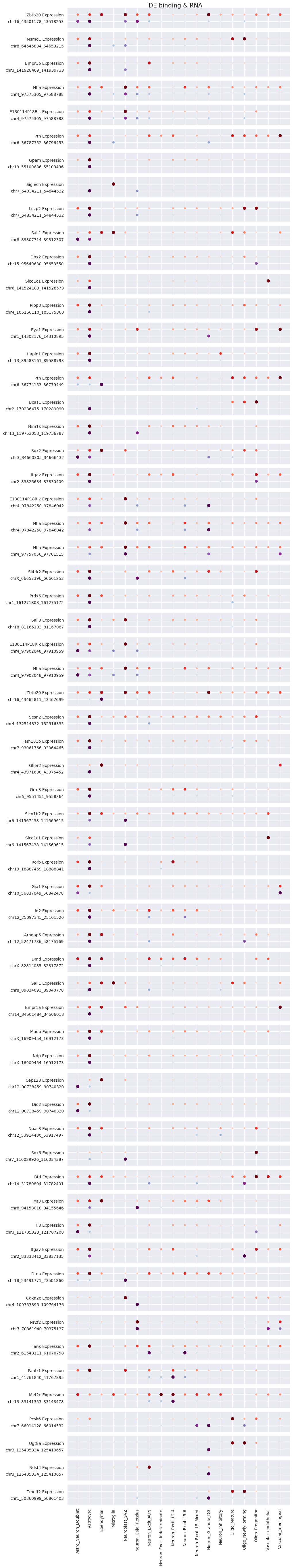
Next, we find peak-gene pairs that are differentially bound/regulated in the specified cell-type. We look at all differential peaks in each cluster and see if the annotated genes are significantly expressed in the cluster. We can then set the pvalue and score/log foldchange cutoff.
[18]:
cc.tl.pair_peak_gene_sc_mu(mdata, pvalue_adj_cutoff_cc = 0.05, pvalue_adj_cutoff_rna = 0.05,
                           lfc_cutoff = 3, score_cutoff = 3)
mdata["CC"].uns['pair']
[18]:
| Cluster | Peak | Logfoldchanges | Pvalue_peak | Pvalue_adj_peak | Gene | Score_gene | Pvalue_gene | Pvalue_adj_gene | Distance_peak_to_gene | |
|---|---|---|---|---|---|---|---|---|---|---|
| 0 | Astrocyte | chr16_43501178_43518253 | 3.077262 | 1.462410e-16 | 2.562874e-14 | Zbtb20 | 79.234276 | 0.000000e+00 | 0.000000e+00 | 0 |
| 1 | Astrocyte | chr8_64645834_64659215 | 4.623955 | 3.114365e-14 | 2.949104e-12 | Msmo1 | 61.964111 | 0.000000e+00 | 0.000000e+00 | 58930 |
| 2 | Astrocyte | chr3_141928409_141939733 | 4.876938 | 3.786296e-14 | 2.949104e-12 | Bmpr1b | 24.131538 | 2.475603e-121 | 1.659753e-120 | 0 |
| 3 | Astrocyte | chr4_97575305_97588788 | 3.099679 | 5.907086e-14 | 4.140867e-12 | Nfia | 45.417362 | 0.000000e+00 | 0.000000e+00 | 188838 |
| 4 | Astrocyte | chr4_97575305_97588788 | 3.099679 | 5.907086e-14 | 4.140867e-12 | E130114P18Rik | 16.893749 | 3.380841e-62 | 1.514206e-61 | 0 |
| ... | ... | ... | ... | ... | ... | ... | ... | ... | ... | ... |
| 57 | Neuron_Excit_L2-4 | chr13_83141353_83148478 | 3.495487 | 3.141216e-06 | 2.446659e-04 | Mef2c | 182.292236 | 0.000000e+00 | 0.000000e+00 | 355556 |
| 58 | Neuron_Excit_L5_Mixed | chr7_66014128_66014532 | 3.737143 | 2.786909e-04 | 2.858012e-02 | Pcsk6 | -16.587570 | 2.263189e-61 | 3.313281e-60 | 0 |
| 59 | Neuron_Granule_DG | chr3_125405334_125410657 | 5.806064 | 1.011677e-04 | 1.251507e-02 | Ugt8a | -23.040115 | 5.201659e-89 | 3.379286e-87 | 454686 |
| 60 | Neuron_Granule_DG | chr3_125405334_125410657 | 5.806064 | 1.011677e-04 | 1.251507e-02 | Ndst4 | 4.497158 | 8.449939e-06 | 3.032315e-05 | 0 |
| 61 | Neuron_Granule_DG | chr1_50860999_50861403 | 4.356917 | 1.071190e-04 | 1.251507e-02 | Tmeff2 | 3.399986 | 7.231398e-04 | 1.952972e-03 | 66120 |
62 rows × 10 columns
Plot the results above to find out the potential relationship between TF bindings and gene expression.
[19]:
cc.pl.dotplot_sc_mu(mdata, figsize=(10, 60))
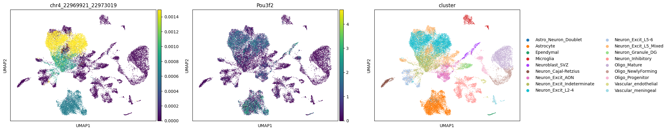
After seeing the dotplot above, bring some peaks to the RNA Anndata object and see the distribution in the UMAP plot.
[20]:
sc.pp.pca(mdata["RNA"])
sc.pp.neighbors(mdata["RNA"])
sc.tl.umap(mdata["RNA"])
The first plot is the average insertions of the peak in each cluster, the second plot is the gene expression Gou3f2 (one of its nearest genes for the peak); the third plot is the cluster information.
[21]:
cc.pl.plot_matched(mdata, 'chr4_22969921_22973019', 'Pou3f2')
/home/juanru/miniconda3/lib/python3.9/site-packages/scanpy/plotting/_tools/scatterplots.py:391: UserWarning: No data for colormapping provided via 'c'. Parameters 'cmap' will be ignored
  cax = scatter(
[22]:
cc.pl.plot_matched(mdata, 'chr1_42253068_42265192', 'Pou3f3')
The history saving thread hit an unexpected error (OperationalError('database is locked')).History will not be written to the database.
/home/juanru/miniconda3/lib/python3.9/site-packages/scanpy/plotting/_tools/scatterplots.py:391: UserWarning: No data for colormapping provided via 'c'. Parameters 'cmap' will be ignored
  cax = scatter(
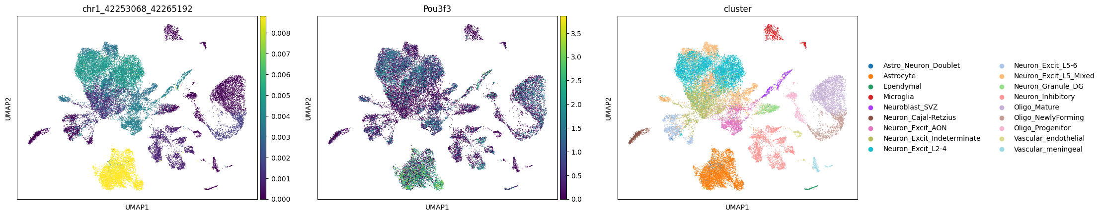
We can see a potential relationship between Brd4 binding and gene expression.
If we map these enhancers to the human genome, are there disease associated SNPs nearby? To answer this question, we can map binding sites and genes to the human genome. We use liftover to get the resuls.
[23]:
mdata["CC"].uns["pair"] = cc.tl.result_mapping(mdata["CC"].uns["pair"])
mdata["CC"].uns["pair"]
Start mapping the peaks to the new genome.
100%|██████████| 62/62 [00:00<00:00, 222.90it/s]
Start finding location of genes in the new genome.
100%|██████████| 62/62 [00:00<00:00, 257.11it/s]
[23]:
| Cluster | Peak | Logfoldchanges | Pvalue_peak | Pvalue_adj_peak | Gene | Score_gene | Pvalue_gene | Pvalue_adj_gene | Distance_peak_to_gene | Chr_liftover | Start_liftover | End_liftover | Chr_hg38 | Start_hg38 | End_hg38 | |
|---|---|---|---|---|---|---|---|---|---|---|---|---|---|---|---|---|
| 0 | Astrocyte | chr16_43501178_43518253 | 3.077262 | 1.462410e-16 | 2.562874e-14 | Zbtb20 | 79.234276 | 0.000000e+00 | 0.000000e+00 | 0 | chr3 | 114439800 | 114457200 | chr3 | 114314499 | 115147280 |
| 1 | Astrocyte | chr8_64645834_64659215 | 4.623955 | 3.114365e-14 | 2.949104e-12 | Msmo1 | 61.964111 | 0.000000e+00 | 0.000000e+00 | 58930 | chr4 | 165418445 | 165438029 | chr4 | 165327665 | 165343162 |
| 2 | Astrocyte | chr3_141928409_141939733 | 4.876938 | 3.786296e-14 | 2.949104e-12 | Bmpr1b | 24.131538 | 2.475603e-121 | 1.659753e-120 | 0 | chr4 | 95040417 | 95054959 | chr4 | 94757976 | 95158450 |
| 3 | Astrocyte | chr4_97575305_97588788 | 3.099679 | 5.907086e-14 | 4.140867e-12 | Nfia | 45.417362 | 0.000000e+00 | 0.000000e+00 | 188838 | chr1 | 60858298 | 60872361 | chr1 | 61077273 | 61462788 |
| 4 | Astrocyte | chr4_97575305_97588788 | 3.099679 | 5.907086e-14 | 4.140867e-12 | E130114P18Rik | 16.893749 | 3.380841e-62 | 1.514206e-61 | 0 | chr1 | 60858298 | 60872361 | |||
| ... | ... | ... | ... | ... | ... | ... | ... | ... | ... | ... | ... | ... | ... | ... | ... | ... |
| 57 | Neuron_Excit_L2-4 | chr13_83141353_83148478 | 3.495487 | 3.141216e-06 | 2.446659e-04 | Mef2c | 182.292236 | 0.000000e+00 | 0.000000e+00 | 355556 | chr5 | 89235156 | 89249323 | chr5 | 88718240 | 88904105 |
| 58 | Neuron_Excit_L5_Mixed | chr7_66014128_66014532 | 3.737143 | 2.786909e-04 | 2.858012e-02 | Pcsk6 | -16.587570 | 2.263189e-61 | 3.313281e-60 | 0 | chr15 | 101337048 | 101337565 | chr15 | 101303927 | 101489984 |
| 59 | Neuron_Granule_DG | chr3_125405334_125410657 | 5.806064 | 1.011677e-04 | 1.251507e-02 | Ugt8a | -23.040115 | 5.201659e-89 | 3.379286e-87 | 454686 | chr4 | 115106106 | 115112630 | |||
| 60 | Neuron_Granule_DG | chr3_125405334_125410657 | 5.806064 | 1.011677e-04 | 1.251507e-02 | Ndst4 | 4.497158 | 8.449939e-06 | 3.032315e-05 | 0 | chr4 | 115106106 | 115112630 | chr4 | 114827772 | 115113876 |
| 61 | Neuron_Granule_DG | chr1_50860999_50861403 | 4.356917 | 1.071190e-04 | 1.251507e-02 | Tmeff2 | 3.399986 | 7.231398e-04 | 1.952972e-03 | 66120 | chr2 | 191949045 | 192194933 |
62 rows × 16 columns
We search the GWAS Catalog database and find out related SNPs in the binding areas.
[24]:
mdata["CC"].uns["pair"] = cc.tl.GWAS(mdata["CC"].uns["pair"])
mdata["CC"].uns["pair"]
[24]:
| Cluster | Peak | Logfoldchanges | Pvalue_peak | Pvalue_adj_peak | Gene | Score_gene | Pvalue_gene | Pvalue_adj_gene | Distance_peak_to_gene | Chr_liftover | Start_liftover | End_liftover | Chr_hg38 | Start_hg38 | End_hg38 | GWAS | |
|---|---|---|---|---|---|---|---|---|---|---|---|---|---|---|---|---|---|
| 0 | Astrocyte | chr16_43501178_43518253 | 3.077262 | 1.462410e-16 | 2.562874e-14 | Zbtb20 | 79.234276 | 0.000000e+00 | 0.000000e+00 | 0 | chr3 | 114439800 | 114457200 | chr3 | 114314499 | 115147280 | Schizophrenia; Smoking status (ever vs never s... |
| 1 | Astrocyte | chr8_64645834_64659215 | 4.623955 | 3.114365e-14 | 2.949104e-12 | Msmo1 | 61.964111 | 0.000000e+00 | 0.000000e+00 | 58930 | chr4 | 165418445 | 165438029 | chr4 | 165327665 | 165343162 | Atopic dermatitis (moderate to severe) |
| 2 | Astrocyte | chr3_141928409_141939733 | 4.876938 | 3.786296e-14 | 2.949104e-12 | Bmpr1b | 24.131538 | 2.475603e-121 | 1.659753e-120 | 0 | chr4 | 95040417 | 95054959 | chr4 | 94757976 | 95158450 | |
| 3 | Astrocyte | chr4_97575305_97588788 | 3.099679 | 5.907086e-14 | 4.140867e-12 | Nfia | 45.417362 | 0.000000e+00 | 0.000000e+00 | 188838 | chr1 | 60858298 | 60872361 | chr1 | 61077273 | 61462788 | Refractive error |
| 4 | Astrocyte | chr4_97575305_97588788 | 3.099679 | 5.907086e-14 | 4.140867e-12 | E130114P18Rik | 16.893749 | 3.380841e-62 | 1.514206e-61 | 0 | chr1 | 60858298 | 60872361 | Refractive error | |||
| ... | ... | ... | ... | ... | ... | ... | ... | ... | ... | ... | ... | ... | ... | ... | ... | ... | ... |
| 57 | Neuron_Excit_L2-4 | chr13_83141353_83148478 | 3.495487 | 3.141216e-06 | 2.446659e-04 | Mef2c | 182.292236 | 0.000000e+00 | 0.000000e+00 | 355556 | chr5 | 89235156 | 89249323 | chr5 | 88718240 | 88904105 | Macular thickness; Waist circumference adjuste... |
| 58 | Neuron_Excit_L5_Mixed | chr7_66014128_66014532 | 3.737143 | 2.786909e-04 | 2.858012e-02 | Pcsk6 | -16.587570 | 2.263189e-61 | 3.313281e-60 | 0 | chr15 | 101337048 | 101337565 | chr15 | 101303927 | 101489984 | |
| 59 | Neuron_Granule_DG | chr3_125405334_125410657 | 5.806064 | 1.011677e-04 | 1.251507e-02 | Ugt8a | -23.040115 | 5.201659e-89 | 3.379286e-87 | 454686 | chr4 | 115106106 | 115112630 | ||||
| 60 | Neuron_Granule_DG | chr3_125405334_125410657 | 5.806064 | 1.011677e-04 | 1.251507e-02 | Ndst4 | 4.497158 | 8.449939e-06 | 3.032315e-05 | 0 | chr4 | 115106106 | 115112630 | chr4 | 114827772 | 115113876 | |
| 61 | Neuron_Granule_DG | chr1_50860999_50861403 | 4.356917 | 1.071190e-04 | 1.251507e-02 | Tmeff2 | 3.399986 | 7.231398e-04 | 1.952972e-03 | 66120 | chr2 | 191949045 | 192194933 |
62 rows × 17 columns
Save the file if needed.
[25]:
mdata.write("Mouse-Cortex.h5mu")