Tutorial: SP1 bindings in Cre-driver mouse lines.
In this tutorial, we will analyze the binding of the transcription factor Sp1, collected using cre-dependant calling cards from a Syn1::Cre-driver mouse line. Bulk unfused (Brd4 directed) data was also collected as backgound. This dataset contains two time points: day 10(P10) and day 28(P28). The dataset is from Cammack et al., PNAS. (2020), and it can be downloaded from GEO.
In this tutorial, we will call peaks, make annotation, and perfrom differential peak analysis. There are 271946 insertions in the SP1 P10 qbed file, 1083099 insertions in the SP1 P28 qbed file, and 5573110 insertions in the brd4 qbed file.
[1]:
import pycallingcards as cc
import numpy as np
import pandas as pd
import scanpy as sc
from matplotlib import pyplot as plt
plt.rcParams['figure.dpi'] = 150
We start by reading the qbed datafile. In this file, each row represents a Sp1-directed insertion and columns indicate the chromosome, start point and end point, read number, the direction and the sample barcode of each insertion. For example, the first row means one insertion is on Chromosome 1, and starts from 3095378 and ends on 3095382. The reads number is 7 with direction going from 3’ to 5’. The barcode of the cell is TAAGG. We give it the group column to distinguish between groups.
Use cc.rd.read_qbed(filename) to read your own qbed data.
[2]:
SP1_P10 = cc.datasets.SP1_Cre_data(data = "SP1_P10")
SP1_P10['group'] = 'P10'
SP1_P10
[2]:
| Chr | Start | End | Reads | Direction | Barcodes | group | |
|---|---|---|---|---|---|---|---|
| 0 | chr1 | 3095378 | 3095382 | 7 | + | TAAGG | P10 |
| 1 | chr1 | 3120128 | 3120132 | 1 | + | GTTAC | P10 |
| 2 | chr1 | 3121275 | 3121279 | 10 | - | GTTAC | P10 |
| 3 | chr1 | 3121275 | 3121279 | 2 | - | GTTAC | P10 |
| 4 | chr1 | 3222947 | 3222951 | 1 | - | GTTAC | P10 |
| ... | ... | ... | ... | ... | ... | ... | ... |
| 271941 | chrY | 1010004 | 1010008 | 1 | - | GTTAC | P10 |
| 271942 | chrY | 1011155 | 1011159 | 12 | - | GTTAC | P10 |
| 271943 | chrY | 1178766 | 1178770 | 10 | + | GTTAC | P10 |
| 271944 | chrY | 1244787 | 1244791 | 11 | + | GTTAC | P10 |
| 271945 | chrY | 5433055 | 5433059 | 2 | + | CGAAA | P10 |
271946 rows × 7 columns
[3]:
SP1_P28 = cc.datasets.SP1_Cre_data(data = "SP1_P28")
SP1_P28['group'] = 'P28'
SP1_P28
[3]:
| Chr | Start | End | Reads | Direction | Barcodes | group | |
|---|---|---|---|---|---|---|---|
| 0 | chr1 | 3071865 | 3071869 | 76 | + | GTCAT | P28 |
| 1 | chr1 | 3095378 | 3095382 | 7 | + | ACTGC | P28 |
| 2 | chr1 | 3102707 | 3102711 | 1 | - | GTCAT | P28 |
| 3 | chr1 | 3119905 | 3119909 | 4 | + | GTCAT | P28 |
| 4 | chr1 | 3120189 | 3120193 | 66 | - | GTCAT | P28 |
| ... | ... | ... | ... | ... | ... | ... | ... |
| 1083094 | chrY | 90803579 | 90803583 | 14 | - | GTCAT | P28 |
| 1083095 | chrY | 90805130 | 90805134 | 10 | + | ACTGC | P28 |
| 1083096 | chrY | 90805130 | 90805134 | 1 | + | CGAAA | P28 |
| 1083097 | chrY | 90806531 | 90806535 | 5 | - | GTCAT | P28 |
| 1083098 | chrY | 90811001 | 90811005 | 63 | + | ACTGC | P28 |
1083099 rows × 7 columns
To call differential peaks, we first combine the two qbed files together.
[4]:
SP1 = cc.rd.combine_qbed([SP1_P10, SP1_P28])
SP1
[4]:
| Chr | Start | End | Reads | Direction | Barcodes | group | |
|---|---|---|---|---|---|---|---|
| 0 | chr1 | 3071865 | 3071869 | 76 | + | GTCAT | P28 |
| 1 | chr1 | 3095378 | 3095382 | 7 | + | TAAGG | P10 |
| 2 | chr1 | 3095378 | 3095382 | 7 | + | ACTGC | P28 |
| 3 | chr1 | 3102707 | 3102711 | 1 | - | GTCAT | P28 |
| 4 | chr1 | 3119905 | 3119909 | 4 | + | GTCAT | P28 |
| ... | ... | ... | ... | ... | ... | ... | ... |
| 1355040 | chrY | 90803579 | 90803583 | 14 | - | GTCAT | P28 |
| 1355041 | chrY | 90805130 | 90805134 | 10 | + | ACTGC | P28 |
| 1355042 | chrY | 90805130 | 90805134 | 1 | + | CGAAA | P28 |
| 1355043 | chrY | 90806531 | 90806535 | 5 | - | GTCAT | P28 |
| 1355044 | chrY | 90811001 | 90811005 | 63 | + | ACTGC | P28 |
1355045 rows × 7 columns
The insertions might be mapped unlocalized or unplaced, we now clean it here.
[5]:
SP1 = cc.pp.clean_qbed(SP1)
SP1
[5]:
| Chr | Start | End | Reads | Direction | Barcodes | group | |
|---|---|---|---|---|---|---|---|
| 0 | chr1 | 3071865 | 3071869 | 76 | + | GTCAT | P28 |
| 1 | chr1 | 3095378 | 3095382 | 7 | + | TAAGG | P10 |
| 2 | chr1 | 3095378 | 3095382 | 7 | + | ACTGC | P28 |
| 3 | chr1 | 3102707 | 3102711 | 1 | - | GTCAT | P28 |
| 4 | chr1 | 3119905 | 3119909 | 4 | + | GTCAT | P28 |
| ... | ... | ... | ... | ... | ... | ... | ... |
| 1355040 | chrY | 90803579 | 90803583 | 14 | - | GTCAT | P28 |
| 1355041 | chrY | 90805130 | 90805134 | 10 | + | ACTGC | P28 |
| 1355042 | chrY | 90805130 | 90805134 | 1 | + | CGAAA | P28 |
| 1355043 | chrY | 90806531 | 90806535 | 5 | - | GTCAT | P28 |
| 1355044 | chrY | 90811001 | 90811005 | 63 | + | ACTGC | P28 |
1354844 rows × 7 columns
We then read the brd4 background file.
[6]:
bg = cc.datasets.SP1_Cre_data(data = "background")
bg
[6]:
| Chr | Start | End | Reads | Direction | Barcodes | |
|---|---|---|---|---|---|---|
| 0 | chr1 | 3004272 | 3004276 | 5 | + | ACTGC |
| 1 | chr1 | 3028063 | 3028067 | 6 | - | ACTGC |
| 2 | chr1 | 3043241 | 3043245 | 1 | - | ACTGC |
| 3 | chr1 | 3049117 | 3049121 | 1 | - | CAGTG |
| 4 | chr1 | 3052152 | 3052156 | 1 | + | ACTGC |
| ... | ... | ... | ... | ... | ... | ... |
| 5573105 | chrY | 90811001 | 90811005 | 2 | + | CAGTG |
| 5573106 | chrY | 90811001 | 90811005 | 1 | + | CAGTG |
| 5573107 | chrY | 90811001 | 90811005 | 1 | + | CAGTG |
| 5573108 | chrY | 90811001 | 90811005 | 2 | + | TGACA |
| 5573109 | chrY | 90811001 | 90811005 | 13 | + | CAGTG |
5573110 rows × 6 columns
[7]:
bg = cc.pp.clean_qbed(bg)
bg
[7]:
| Chr | Start | End | Reads | Direction | Barcodes | |
|---|---|---|---|---|---|---|
| 0 | chr1 | 3004272 | 3004276 | 5 | + | ACTGC |
| 1 | chr1 | 3028063 | 3028067 | 6 | - | ACTGC |
| 2 | chr1 | 3043241 | 3043245 | 1 | - | ACTGC |
| 3 | chr1 | 3049117 | 3049121 | 1 | - | CAGTG |
| 4 | chr1 | 3052152 | 3052156 | 1 | + | ACTGC |
| ... | ... | ... | ... | ... | ... | ... |
| 5573105 | chrY | 90811001 | 90811005 | 2 | + | CAGTG |
| 5573106 | chrY | 90811001 | 90811005 | 1 | + | CAGTG |
| 5573107 | chrY | 90811001 | 90811005 | 1 | + | CAGTG |
| 5573108 | chrY | 90811001 | 90811005 | 2 | + | TGACA |
| 5573109 | chrY | 90811001 | 90811005 | 13 | + | CAGTG |
5572856 rows × 6 columns
We next need to call peaks to identify potential Sp1 binding sites. Three different methods (‘CCcaller’, ‘MACCs’, ‘Blockify’) are available along with three different species (‘hg38’, ‘mm10’, ‘sacCer3’).
Here, we use MACCs in mouse(‘mm10’) data. window_size is the most important parameter for MACCs, and it is highly related to the length of a peak. 1000-1200 is a good fit for window_size. step_size is another important parameter and it controls how careful we are looking into the chromosomes. 500-800 is good for step_size. pvalue_cutoffTTAA is the pvalue cutoff for TTAA data and pvalue_cutoffbg is pvalue cutoff for the background qbed data. Normally, the setting for pvalue_cutoffbg is considerably higher than pvalue_cutoffTTAA. pvalue_cutoffbg is recommended from 0.00001 to 0.01 and pvalue_cutoffTTAA is recommended from 0.001 to 0.1. The setting of pseudocounts is largely influenced by library size. For the first time of trial, it can be adjusted to \(10^{6}-10^{-5} \times\) the number of insertions.
[8]:
peak_data = cc.pp.call_peaks(SP1, bg, method = "MACCs", reference = "mm10", pvalue_cutoffbg = 0.001,
                             window_size = 1000, step_size = 500, pvalue_cutoffTTAA = 0.00001,
                             lam_win_size = 1000000, pseudocounts = 0.1, record = True, save = "peak.bed")
peak_data
For the MACCs method with background, [expdata, background, reference, pvalue_cutoffbg, pvalue_cutoffTTAA, lam_win_size, window_size, step_size, extend, pseudocounts, test_method, min_insertions, record] would be utilized.
100%|██████████| 21/21 [04:43<00:00, 13.50s/it]
[8]:
| Chr | Start | End | Center | Experiment Insertions | Background insertions | Reference Insertions | pvalue Reference | pvalue Background | Fraction Experiment | TPH Experiment | Fraction background | TPH background | TPH background subtracted | pvalue_adj Reference | |
|---|---|---|---|---|---|---|---|---|---|---|---|---|---|---|---|
| 0 | chr1 | 3399656 | 3400345 | 3400068.0 | 21 | 69 | 8 | 0.000000e+00 | 1.745466e-04 | 0.000015 | 1549.993948 | 1.238144e-05 | 1238.144320 | 311.849628 | 0.000000e+00 |
| 1 | chr1 | 3672013 | 3673193 | 3672213.0 | 61 | 47 | 9 | 0.000000e+00 | 0.000000e+00 | 0.000045 | 4502.363372 | 8.433737e-06 | 843.373667 | 3658.989705 | 0.000000e+00 |
| 2 | chr1 | 4773450 | 4774236 | 4773657.0 | 6 | 5 | 4 | 2.405425e-08 | 1.939280e-04 | 0.000004 | 442.855414 | 8.972060e-07 | 89.720603 | 353.134811 | 6.323087e-06 |
| 3 | chr1 | 4785206 | 4786550 | 4785472.0 | 31 | 47 | 13 | 0.000000e+00 | 2.298502e-08 | 0.000023 | 2288.086304 | 8.433737e-06 | 843.373667 | 1444.712637 | 0.000000e+00 |
| 4 | chr1 | 5016489 | 5017564 | 5017023.0 | 8 | 10 | 8 | 1.672281e-09 | 3.938477e-04 | 0.000006 | 590.473885 | 1.794412e-06 | 179.441206 | 411.032679 | 4.739980e-07 |
| ... | ... | ... | ... | ... | ... | ... | ... | ... | ... | ... | ... | ... | ... | ... | ... |
| 10739 | chrX | 169325223 | 169325838 | 169325423.0 | 11 | 16 | 9 | 5.107026e-15 | 1.876575e-04 | 0.000008 | 811.901592 | 2.871059e-06 | 287.105929 | 524.795662 | 1.893816e-12 |
| 10740 | chrX | 169799382 | 169801491 | 169799905.0 | 25 | 29 | 23 | 0.000000e+00 | 3.271381e-07 | 0.000018 | 1845.230890 | 5.203795e-06 | 520.379497 | 1324.851393 | 0.000000e+00 |
| 10741 | chrX | 169829316 | 169830343 | 169829658.0 | 9 | 9 | 10 | 2.746225e-09 | 1.659074e-04 | 0.000007 | 664.283120 | 1.614971e-06 | 161.497085 | 502.786035 | 7.671705e-07 |
| 10742 | chrX | 169878786 | 169879561 | 169879328.0 | 19 | 21 | 10 | 0.000000e+00 | 1.379092e-06 | 0.000014 | 1402.375476 | 3.768265e-06 | 376.826532 | 1025.548944 | 0.000000e+00 |
| 10743 | chrY | 1009804 | 1011442 | 1010850.0 | 17 | 2 | 16 | 0.000000e+00 | 7.771561e-16 | 0.000013 | 1254.757005 | 3.588824e-07 | 35.888241 | 1218.868764 | 0.000000e+00 |
10744 rows × 15 columns
Approach the above by first combining the data and then call peaks together.
Although not recommended, you could also try calling peaks seperately and then merging the peaks by pybedtools. Below is the code:
import pybedtools
peak_data1 = cc.pp.call_peaks(SP1_P10, bg, method = "MACCs", reference = "mm10",
                              pvalue_cutoffbg = 0.1, window_size=1500, step_size=500,
                              lam_win_size = None,  pseudocounts = 0.1, record = True)
peak_data2 = cc.pp.call_peaks(SP1_P28, bg, method = "MACCs", reference = "mm10",
                              pvalue_cutoffbg = 0.1, window_size=1500, step_size=500,
                              lam_win_size = None,  pseudocounts = 0.1, record = True)
peak = cc.rd.combine_qbed([peak_data1, peak_data2])
peak = pybedtools.BedTool.from_dataframe(peak).merge().to_dataframe()
peak_data = peak.rename(columns={"chrom":"Chr", "start":"Start", "end":"End"})
In order to choose the suitable method and parameters for peak calling, please take a look at genome areas. We stongly advise to adjust the parameters for cc.pp.call_peaks() to call better peaks.
In this plot, the colored ones are the experiment qbed data and the gray ones are the background data. The top section shows insertions and their read counts. One dot is an insertion and the height is log(reads+1). The middle section indicates the distribution of insertions. The bottom section represents reference genes and peaks.
[9]:
cc.pl.draw_area("chr1", 4856929, 4863861, 100000, peak_data, SP1, "mm10", bg, font_size=2, plotsize = [1,1,6],
                figsize = (30,12), peak_line = 2, save = False, bins = 500, example_length = 5000)
[10]:
cc.pl.draw_area("chr2", 3116481, 3125943, 15000, peak_data, SP1, "mm10", bg, font_size=2, plotsize = [1,1,3],
                figsize = (30,10), peak_line = 3, save = False, bins = 500, example_length = 1000)
We can also visualize our data directly in the WashU Epigenome Browser. This can be useful for overlaying your data with other published datasets. Please note that this link only valid for 24hrs, so you will have to rerun it if you want to use it after this time period.
[11]:
qbed= {"SP1":SP1, "bg":bg}
bed = {'PEAK':peak_data}
cc.pl.WashU_browser_url(qbed, bed, genome = 'mm10')
All qbed addressed
All bed addressed
Uploading files
Please click the following link to see the data on WashU Epigenome Browser directly.
https://epigenomegateway.wustl.edu/browser/?genome=mm10&hub=https://companion.epigenomegateway.org//task/a4f06270936d67281d4c9aa3065922e2/output//datahub.json
Pycallingcards can be used to visual peak locations acorss the genome to see that the distribution of peaks is unbiased and that all chromosomes are represented.
[12]:
cc.pl.whole_peaks(peak_data, linewidth = 1, reference = "mm10")
We can next use HOMER to look for motifs that are overrepresented under the peaks. Here, we expect to find the SP1 motif.
[13]:
cc.tl.call_motif(peaks_frame = peak_data, reference = "mm10", save_homer = "Homer/peak",
                 homer_path = "/home/juanru/miniconda3/bin/", num_cores=12)
There is no save_name, it will save to temp_Homer_trial.bed and then delete.
        Position file = temp_Homer_trial.bed
        Genome = mm10
        Output Directory = Homer/peak
        Fragment size set to 1000
        Using 12 CPUs
        Will not run homer for de novo motifs
        Found mset for "mouse", will check against vertebrates motifs
        Peak/BED file conversion summary:
                BED/Header formatted lines: 10744
                peakfile formatted lines: 0

        Peak File Statistics:
                Total Peaks: 10744
                Redundant Peak IDs: 0
                Peaks lacking information: 0 (need at least 5 columns per peak)
                Peaks with misformatted coordinates: 0 (should be integer)
                Peaks with misformatted strand: 0 (should be either +/- or 0/1)

        Peak file looks good!

        Background files for 1000 bp fragments found.
        Custom genome sequence directory: /home/juanru/miniconda3/share/homer/.//data/genomes/mm10//

        Extracting sequences from directory: /home/juanru/miniconda3/share/homer/.//data/genomes/mm10//
        Extracting 680 sequences from chr1
        Extracting 873 sequences from chr2
        Extracting 561 sequences from chr3
        Extracting 698 sequences from chr4
        Extracting 682 sequences from chr5
        Extracting 540 sequences from chr6
        Extracting 670 sequences from chr7
        Extracting 535 sequences from chr8
        Extracting 609 sequences from chr9
        Extracting 557 sequences from chr10
        Extracting 768 sequences from chr11
        Extracting 469 sequences from chr12
        Extracting 427 sequences from chr13
        Extracting 413 sequences from chr14
        Extracting 422 sequences from chr15
        Extracting 396 sequences from chr16
        Extracting 453 sequences from chr17
        Extracting 366 sequences from chr18
        Extracting 325 sequences from chr19
        Extracting 299 sequences from chrX
        Extracting 1 sequences from chrY
                1 of 10744 removed because they had >70.00% Ns (i.e. masked repeats)

        Not removing redundant sequences


        Sequences processed:
                Auto detected maximum sequence length of 1001 bp
                10743 total

        Frequency Bins: 0.2 0.25 0.3 0.35 0.4 0.45 0.5 0.6 0.7 0.8
        Freq    Bin     Count
        0.3     2       6
        0.35    3       180
        0.4     4       932
        0.45    5       2120
        0.5     6       2862
        0.6     7       3871
        0.7     8       717
        0.8     9       55

        Total sequences set to 50000

        Choosing background that matches in CpG/GC content...
        Bin     # Targets       # Background    Background Weight
        2       6       22      0.997
        3       180     658     1.000
        4       932     3406    1.000
        5       2120    7747    1.000
        6       2862    10458   1.000
        7       3871    14145   1.000
        8       717     2620    1.000
        9       55      201     1.000
        Assembling sequence file...
        Normalizing lower order oligos using homer2

        Reading input files...
        50000 total sequences read
        Autonormalization: 1-mers (4 total)
                A       25.47%  25.72%  0.990
                C       24.53%  24.28%  1.010
                G       24.53%  24.28%  1.010
                T       25.47%  25.72%  0.990
        Autonormalization: 2-mers (16 total)
                AA      7.69%   7.08%   1.087
                CA      6.98%   7.64%   0.914
                GA      6.16%   6.34%   0.972
                TA      4.64%   4.66%   0.996
                AC      5.10%   5.36%   0.951
                CC      7.22%   7.02%   1.029
                GC      6.05%   5.57%   1.087
                TC      6.16%   6.34%   0.972
                AG      7.55%   7.89%   0.957
                CG      2.78%   1.74%   1.598
                GG      7.22%   7.02%   1.029
                TG      6.98%   7.64%   0.914
                AT      5.13%   5.38%   0.953
                CT      7.55%   7.89%   0.957
                GT      5.10%   5.36%   0.951
                TT      7.69%   7.08%   1.087
        Autonormalization: 3-mers (64 total)
        Normalization weights can be found in file: Homer/peak/seq.autonorm.tsv
        Converging on autonormalization solution:
        ...............................................................................
        Final normalization:    Autonormalization: 1-mers (4 total)
                A       25.47%  25.41%  1.002
                C       24.53%  24.59%  0.998
                G       24.53%  24.59%  0.998
                T       25.47%  25.41%  1.002
        Autonormalization: 2-mers (16 total)
                AA      7.69%   7.40%   1.040
                CA      6.98%   7.14%   0.977
                GA      6.16%   6.21%   0.992
                TA      4.64%   4.67%   0.995
                AC      5.10%   5.16%   0.989
                CC      7.22%   7.21%   1.001
                GC      6.05%   6.01%   1.007
                TC      6.16%   6.21%   0.992
                AG      7.55%   7.58%   0.996
                CG      2.78%   2.65%   1.049
                GG      7.22%   7.21%   1.001
                TG      6.98%   7.14%   0.977
                AT      5.13%   5.28%   0.972
                CT      7.55%   7.58%   0.996
                GT      5.10%   5.16%   0.989
                TT      7.69%   7.40%   1.040
        Autonormalization: 3-mers (64 total)
        Finished preparing sequence/group files

        ----------------------------------------------------------
        Known motif enrichment

        Reading input files...
        50000 total sequences read
        440 motifs loaded
        Cache length = 11180
        Using binomial scoring
        Checking enrichment of 440 motif(s)
        |0%                                    50%                                  100%|
        =================================================================================
Finished!
        Preparing HTML output with sequence logos...
                1 of 440 (1e-529) Sp5(Zf)/mES-Sp5.Flag-ChIP-Seq(GSE72989)/Homer
                2 of 440 (1e-371) Sp2(Zf)/HEK293-Sp2.eGFP-ChIP-Seq(Encode)/Homer
                3 of 440 (1e-365) KLF14(Zf)/HEK293-KLF14.GFP-ChIP-Seq(GSE58341)/Homer
                4 of 440 (1e-354) KLF1(Zf)/HUDEP2-KLF1-CutnRun(GSE136251)/Homer
                5 of 440 (1e-294) Sp1(Zf)/Promoter/Homer
                6 of 440 (1e-258) KLF3(Zf)/MEF-Klf3-ChIP-Seq(GSE44748)/Homer
                7 of 440 (1e-251) Maz(Zf)/HepG2-Maz-ChIP-Seq(GSE31477)/Homer
                8 of 440 (1e-229) KLF5(Zf)/LoVo-KLF5-ChIP-Seq(GSE49402)/Homer
                9 of 440 (1e-221) KLF6(Zf)/PDAC-KLF6-ChIP-Seq(GSE64557)/Homer
                10 of 440 (1e-154) Klf9(Zf)/GBM-Klf9-ChIP-Seq(GSE62211)/Homer
                11 of 440 (1e-110) Klf4(Zf)/mES-Klf4-ChIP-Seq(GSE11431)/Homer
                12 of 440 (1e-94) TATA-Box(TBP)/Promoter/Homer
                13 of 440 (1e-74) KLF10(Zf)/HEK293-KLF10.GFP-ChIP-Seq(GSE58341)/Homer
                14 of 440 (1e-63) Egr1(Zf)/K562-Egr1-ChIP-Seq(GSE32465)/Homer
                15 of 440 (1e-58) E2F3(E2F)/MEF-E2F3-ChIP-Seq(GSE71376)/Homer
                16 of 440 (1e-53) Zfp281(Zf)/ES-Zfp281-ChIP-Seq(GSE81042)/Homer
                17 of 440 (1e-52) WT1(Zf)/Kidney-WT1-ChIP-Seq(GSE90016)/Homer
                18 of 440 (1e-50) Lhx3(Homeobox)/Neuron-Lhx3-ChIP-Seq(GSE31456)/Homer
                19 of 440 (1e-47) Nkx6.1(Homeobox)/Islet-Nkx6.1-ChIP-Seq(GSE40975)/Homer
                20 of 440 (1e-47) ZNF467(Zf)/HEK293-ZNF467.GFP-ChIP-Seq(GSE58341)/Homer
                21 of 440 (1e-45) RFX(HTH)/K562-RFX3-ChIP-Seq(SRA012198)/Homer
                22 of 440 (1e-43) Znf263(Zf)/K562-Znf263-ChIP-Seq(GSE31477)/Homer
                23 of 440 (1e-42) Hoxa13(Homeobox)/ChickenMSG-Hoxa13.Flag-ChIP-Seq(GSE86088)/Homer
                24 of 440 (1e-40) Lhx1(Homeobox)/EmbryoCarcinoma-Lhx1-ChIP-Seq(GSE70957)/Homer
                25 of 440 (1e-39) Mef2c(MADS)/GM12878-Mef2c-ChIP-Seq(GSE32465)/Homer
                26 of 440 (1e-38) CHR(?)/Hela-CellCycle-Expression/Homer
                27 of 440 (1e-37) Rfx2(HTH)/LoVo-RFX2-ChIP-Seq(GSE49402)/Homer
                28 of 440 (1e-37) Isl1(Homeobox)/Neuron-Isl1-ChIP-Seq(GSE31456)/Homer
                29 of 440 (1e-37) Dlx3(Homeobox)/Kerainocytes-Dlx3-ChIP-Seq(GSE89884)/Homer
                30 of 440 (1e-36) En1(Homeobox)/SUM149-EN1-ChIP-Seq(GSE120957)/Homer
                31 of 440 (1e-36) X-box(HTH)/NPC-H3K4me1-ChIP-Seq(GSE16256)/Homer
                32 of 440 (1e-35) Mef2d(MADS)/Retina-Mef2d-ChIP-Seq(GSE61391)/Homer
                33 of 440 (1e-33) E2F6(E2F)/Hela-E2F6-ChIP-Seq(GSE31477)/Homer
                34 of 440 (1e-33) DLX5(Homeobox)/BasalGanglia-Dlx5-ChIP-seq(GSE124936)/Homer
                35 of 440 (1e-32) LHX9(Homeobox)/Hct116-LHX9.V5-ChIP-Seq(GSE116822)/Homer
                36 of 440 (1e-31) E2F4(E2F)/K562-E2F4-ChIP-Seq(GSE31477)/Homer
                37 of 440 (1e-31) EKLF(Zf)/Erythrocyte-Klf1-ChIP-Seq(GSE20478)/Homer
                38 of 440 (1e-31) BMYB(HTH)/Hela-BMYB-ChIP-Seq(GSE27030)/Homer
                39 of 440 (1e-30) DLX2(Homeobox)/BasalGanglia-Dlx2-ChIP-seq(GSE124936)/Homer
                40 of 440 (1e-30) Lhx2(Homeobox)/HFSC-Lhx2-ChIP-Seq(GSE48068)/Homer
                41 of 440 (1e-29) Pitx1(Homeobox)/Chicken-Pitx1-ChIP-Seq(GSE38910)/Homer
                42 of 440 (1e-28) Mef2b(MADS)/HEK293-Mef2b.V5-ChIP-Seq(GSE67450)/Homer
                43 of 440 (1e-28) Elk4(ETS)/Hela-Elk4-ChIP-Seq(GSE31477)/Homer
                44 of 440 (1e-27) DLX1(Homeobox)/BasalGanglia-Dlx1-ChIP-seq(GSE124936)/Homer
                45 of 440 (1e-25) Hoxa11(Homeobox)/ChickenMSG-Hoxa11.Flag-ChIP-Seq(GSE86088)/Homer
                46 of 440 (1e-25) Hoxd13(Homeobox)/ChickenMSG-Hoxd13.Flag-ChIP-Seq(GSE86088)/Homer
                47 of 440 (1e-23) Hoxd11(Homeobox)/ChickenMSG-Hoxd11.Flag-ChIP-Seq(GSE86088)/Homer
                48 of 440 (1e-23) Unknown(Homeobox)/Limb-p300-ChIP-Seq/Homer
                49 of 440 (1e-22) MYB(HTH)/ERMYB-Myb-ChIPSeq(GSE22095)/Homer
                50 of 440 (1e-21) Rfx1(HTH)/NPC-H3K4me1-ChIP-Seq(GSE16256)/Homer
                51 of 440 (1e-19) Nanog(Homeobox)/mES-Nanog-ChIP-Seq(GSE11724)/Homer
                52 of 440 (1e-18) Mef2a(MADS)/HL1-Mef2a.biotin-ChIP-Seq(GSE21529)/Homer
                53 of 440 (1e-18) Arnt:Ahr(bHLH)/MCF7-Arnt-ChIP-Seq(Lo_et_al.)/Homer
                54 of 440 (1e-18) HIF-1b(HLH)/T47D-HIF1b-ChIP-Seq(GSE59937)/Homer
                55 of 440 (1e-17) Gfi1b(Zf)/HPC7-Gfi1b-ChIP-Seq(GSE22178)/Homer
                56 of 440 (1e-17) Egr2(Zf)/Thymocytes-Egr2-ChIP-Seq(GSE34254)/Homer
                57 of 440 (1e-17) Npas4(bHLH)/Neuron-Npas4-ChIP-Seq(GSE127793)/Homer
                58 of 440 (1e-16) CTCF(Zf)/CD4+-CTCF-ChIP-Seq(Barski_et_al.)/Homer
                59 of 440 (1e-14) CEBP(bZIP)/ThioMac-CEBPb-ChIP-Seq(GSE21512)/Homer
                60 of 440 (1e-14) Tbr1(T-box)/Cortex-Tbr1-ChIP-Seq(GSE71384)/Homer
                61 of 440 (1e-13) Elk1(ETS)/Hela-Elk1-ChIP-Seq(GSE31477)/Homer
                62 of 440 (1e-13) Fli1(ETS)/CD8-FLI-ChIP-Seq(GSE20898)/Homer
                63 of 440 (1e-12) AMYB(HTH)/Testes-AMYB-ChIP-Seq(GSE44588)/Homer
                64 of 440 (1e-12) Tcf12(bHLH)/GM12878-Tcf12-ChIP-Seq(GSE32465)/Homer
                65 of 440 (1e-11) JunD(bZIP)/K562-JunD-ChIP-Seq/Homer
                66 of 440 (1e-11) Oct11(POU,Homeobox)/NCIH1048-POU2F3-ChIP-seq(GSE115123)/Homer
                67 of 440 (1e-11) ETV4(ETS)/HepG2-ETV4-ChIP-Seq(ENCODE)/Homer
                68 of 440 (1e-11) STAT6(Stat)/Macrophage-Stat6-ChIP-Seq(GSE38377)/Homer
                69 of 440 (1e-10) CRX(Homeobox)/Retina-Crx-ChIP-Seq(GSE20012)/Homer
                70 of 440 (1e-10) Ronin(THAP)/ES-Thap11-ChIP-Seq(GSE51522)/Homer
                71 of 440 (1e-9) Rbpj1(?)/Panc1-Rbpj1-ChIP-Seq(GSE47459)/Homer
                72 of 440 (1e-9) MYNN(Zf)/HEK293-MYNN.eGFP-ChIP-Seq(Encode)/Homer
                73 of 440 (1e-9) Hnf1(Homeobox)/Liver-Foxa2-Chip-Seq(GSE25694)/Homer
                74 of 440 (1e-9) Myf5(bHLH)/GM-Myf5-ChIP-Seq(GSE24852)/Homer
                75 of 440 (1e-8) Hoxa9(Homeobox)/ChickenMSG-Hoxa9.Flag-ChIP-Seq(GSE86088)/Homer
                76 of 440 (1e-8) HIF2a(bHLH)/785_O-HIF2a-ChIP-Seq(GSE34871)/Homer
                77 of 440 (1e-8) ELF1(ETS)/Jurkat-ELF1-ChIP-Seq(SRA014231)/Homer
                78 of 440 (1e-8) NFY(CCAAT)/Promoter/Homer
                79 of 440 (1e-8) Hoxc9(Homeobox)/Ainv15-Hoxc9-ChIP-Seq(GSE21812)/Homer
                80 of 440 (1e-8) Zfp57(Zf)/H1-ZFP57.HA-ChIP-Seq(GSE115387)/Homer
                81 of 440 (1e-8) NF1-halfsite(CTF)/LNCaP-NF1-ChIP-Seq(Unpublished)/Homer
                82 of 440 (1e-7) Nkx2.2(Homeobox)/NPC-Nkx2.2-ChIP-Seq(GSE61673)/Homer
                83 of 440 (1e-7) GFY(?)/Promoter/Homer
                84 of 440 (1e-7) MyoD(bHLH)/Myotube-MyoD-ChIP-Seq(GSE21614)/Homer
                85 of 440 (1e-7) Stat3+il21(Stat)/CD4-Stat3-ChIP-Seq(GSE19198)/Homer
                86 of 440 (1e-7) STAT6(Stat)/CD4-Stat6-ChIP-Seq(GSE22104)/Homer
                87 of 440 (1e-7) FoxD3(forkhead)/ZebrafishEmbryo-Foxd3.biotin-ChIP-seq(GSE106676)/Homer
                88 of 440 (1e-6) Rfx6(HTH)/Min6b1-Rfx6.HA-ChIP-Seq(GSE62844)/Homer
                89 of 440 (1e-6) E2F1(E2F)/Hela-E2F1-ChIP-Seq(GSE22478)/Homer
                90 of 440 (1e-6) Prop1(Homeobox)/GHFT1-PROP1.biotin-ChIP-Seq(GSE77302)/Homer
                91 of 440 (1e-6) STAT4(Stat)/CD4-Stat4-ChIP-Seq(GSE22104)/Homer
                92 of 440 (1e-6) Tcf21(bHLH)/ArterySmoothMuscle-Tcf21-ChIP-Seq(GSE61369)/Homer
                93 of 440 (1e-6) GLIS3(Zf)/Thyroid-Glis3.GFP-ChIP-Seq(GSE103297)/Homer
                94 of 440 (1e-6) Eomes(T-box)/H9-Eomes-ChIP-Seq(GSE26097)/Homer
                95 of 440 (1e-6) Stat3(Stat)/mES-Stat3-ChIP-Seq(GSE11431)/Homer
                96 of 440 (1e-6) NRF1(NRF)/MCF7-NRF1-ChIP-Seq(Unpublished)/Homer
                97 of 440 (1e-6) ZNF652/HepG2-ZNF652.Flag-ChIP-Seq(Encode)/Homer
                98 of 440 (1e-5) Rfx5(HTH)/GM12878-Rfx5-ChIP-Seq(GSE31477)/Homer
                99 of 440 (1e-5) RORg(NR)/Liver-Rorc-ChIP-Seq(GSE101115)/Homer
                100 of 440 (1e-5) NFAT(RHD)/Jurkat-NFATC1-ChIP-Seq(Jolma_et_al.)/Homer
                101 of 440 (1e-5) Ap4(bHLH)/AML-Tfap4-ChIP-Seq(GSE45738)/Homer
                102 of 440 (1e-5) Fox:Ebox(Forkhead,bHLH)/Panc1-Foxa2-ChIP-Seq(GSE47459)/Homer
                103 of 440 (1e-5) Pitx1:Ebox(Homeobox,bHLH)/Hindlimb-Pitx1-ChIP-Seq(GSE41591)/Homer
                104 of 440 (1e-5) MyoG(bHLH)/C2C12-MyoG-ChIP-Seq(GSE36024)/Homer
                105 of 440 (1e-5) ETV1(ETS)/GIST48-ETV1-ChIP-Seq(GSE22441)/Homer
                106 of 440 (1e-5) NFIL3(bZIP)/HepG2-NFIL3-ChIP-Seq(Encode)/Homer
                107 of 440 (1e-5) NRF(NRF)/Promoter/Homer
                108 of 440 (1e-5) Fos(bZIP)/TSC-Fos-ChIP-Seq(GSE110950)/Homer
                109 of 440 (1e-4) TEAD1(TEAD)/HepG2-TEAD1-ChIP-Seq(Encode)/Homer
                110 of 440 (1e-4) HLF(bZIP)/HSC-HLF.Flag-ChIP-Seq(GSE69817)/Homer
                111 of 440 (1e-4) Tbx5(T-box)/HL1-Tbx5.biotin-ChIP-Seq(GSE21529)/Homer
                112 of 440 (1e-4) NFkB-p65(RHD)/GM12787-p65-ChIP-Seq(GSE19485)/Homer
                113 of 440 (1e-4) HNF1b(Homeobox)/PDAC-HNF1B-ChIP-Seq(GSE64557)/Homer
                114 of 440 (1e-4) BORIS(Zf)/K562-CTCFL-ChIP-Seq(GSE32465)/Homer
                115 of 440 (1e-4) E2F7(E2F)/Hela-E2F7-ChIP-Seq(GSE32673)/Homer
                116 of 440 (1e-4) CRE(bZIP)/Promoter/Homer
                117 of 440 (1e-4) GABPA(ETS)/Jurkat-GABPa-ChIP-Seq(GSE17954)/Homer
                118 of 440 (1e-4) ERG(ETS)/VCaP-ERG-ChIP-Seq(GSE14097)/Homer
                119 of 440 (1e-4) Smad3(MAD)/NPC-Smad3-ChIP-Seq(GSE36673)/Homer
                120 of 440 (1e-4) HIC1(Zf)/Treg-ZBTB29-ChIP-Seq(GSE99889)/Homer
                121 of 440 (1e-4) HOXB13(Homeobox)/ProstateTumor-HOXB13-ChIP-Seq(GSE56288)/Homer
                122 of 440 (1e-4) Hoxd12(Homeobox)/ChickenMSG-Hoxd12.Flag-ChIP-Seq(GSE86088)/Homer
                123 of 440 (1e-4) c-Myc(bHLH)/LNCAP-cMyc-ChIP-Seq(Unpublished)/Homer
                124 of 440 (1e-4) CArG(MADS)/PUER-Srf-ChIP-Seq(Sullivan_et_al.)/Homer
                125 of 440 (1e-4) TEAD3(TEA)/HepG2-TEAD3-ChIP-Seq(Encode)/Homer
                126 of 440 (1e-4) Oct4:Sox17(POU,Homeobox,HMG)/F9-Sox17-ChIP-Seq(GSE44553)/Homer
                127 of 440 (1e-4) OCT:OCT(POU,Homeobox)/NPC-Brn1-ChIP-Seq(GSE35496)/Homer
                128 of 440 (1e-4) Foxo3(Forkhead)/U2OS-Foxo3-ChIP-Seq(E-MTAB-2701)/Homer
                129 of 440 (1e-4) STAT5(Stat)/mCD4+-Stat5-ChIP-Seq(GSE12346)/Homer
                130 of 440 (1e-4) FOXA1(Forkhead)/LNCAP-FOXA1-ChIP-Seq(GSE27824)/Homer
                131 of 440 (1e-4) HIF-1a(bHLH)/MCF7-HIF1a-ChIP-Seq(GSE28352)/Homer
                132 of 440 (1e-3) PBX2(Homeobox)/K562-PBX2-ChIP-Seq(Encode)/Homer
                133 of 440 (1e-3) Phox2a(Homeobox)/Neuron-Phox2a-ChIP-Seq(GSE31456)/Homer
                134 of 440 (1e-3) ZSCAN22(Zf)/HEK293-ZSCAN22.GFP-ChIP-Seq(GSE58341)/Homer
                135 of 440 (1e-3) Atoh1(bHLH)/Cerebellum-Atoh1-ChIP-Seq(GSE22111)/Homer
                136 of 440 (1e-3) RORa(NR)/Liver-Rora-ChIP-Seq(GSE101115)/Homer
                137 of 440 (1e-3) OCT:OCT(POU,Homeobox,IR1)/NPC-Brn2-ChIP-Seq(GSE35496)/Homer
                138 of 440 (1e-3) PRDM15(Zf)/ESC-Prdm15-ChIP-Seq(GSE73694)/Homer
                139 of 440 (1e-3) Fra2(bZIP)/Striatum-Fra2-ChIP-Seq(GSE43429)/Homer
                140 of 440 (1e-3) PU.1-IRF(ETS:IRF)/Bcell-PU.1-ChIP-Seq(GSE21512)/Homer
                141 of 440 (1e-3) Atf2(bZIP)/3T3L1-Atf2-ChIP-Seq(GSE56872)/Homer
                142 of 440 (1e-3) c-Jun-CRE(bZIP)/K562-cJun-ChIP-Seq(GSE31477)/Homer
                143 of 440 (1e-3) OCT:OCT-short(POU,Homeobox)/NPC-OCT6-ChIP-Seq(GSE43916)/Homer
                144 of 440 (1e-3) CEBP:AP1(bZIP)/ThioMac-CEBPb-ChIP-Seq(GSE21512)/Homer
                145 of 440 (1e-3) Oct4(POU,Homeobox)/mES-Oct4-ChIP-Seq(GSE11431)/Homer
                146 of 440 (1e-3) Fra1(bZIP)/BT549-Fra1-ChIP-Seq(GSE46166)/Homer
                147 of 440 (1e-3) Pit1(Homeobox)/GCrat-Pit1-ChIP-Seq(GSE58009)/Homer
                148 of 440 (1e-3) Atf1(bZIP)/K562-ATF1-ChIP-Seq(GSE31477)/Homer
                149 of 440 (1e-3) E-box(bHLH)/Promoter/Homer
                150 of 440 (1e-2) Smad4(MAD)/ESC-SMAD4-ChIP-Seq(GSE29422)/Homer
                151 of 440 (1e-2) STAT1(Stat)/HelaS3-STAT1-ChIP-Seq(GSE12782)/Homer
                152 of 440 (1e-2) Jun-AP1(bZIP)/K562-cJun-ChIP-Seq(GSE31477)/Homer
                153 of 440 (1e-2) FOXA1(Forkhead)/MCF7-FOXA1-ChIP-Seq(GSE26831)/Homer
                154 of 440 (1e-2) JunB(bZIP)/DendriticCells-Junb-ChIP-Seq(GSE36099)/Homer
                155 of 440 (1e-2) IRF3(IRF)/BMDM-Irf3-ChIP-Seq(GSE67343)/Homer
                156 of 440 (1e-2) ZNF675(Zf)/HEK293-ZNF675.GFP-ChIP-Seq(GSE58341)/Homer
                157 of 440 (1e-2) GSC(Homeobox)/FrogEmbryos-GSC-ChIP-Seq(DRA000576)/Homer
                158 of 440 (1e-2) Brn1(POU,Homeobox)/NPC-Brn1-ChIP-Seq(GSE35496)/Homer
                159 of 440 (1e-2) Fosl2(bZIP)/3T3L1-Fosl2-ChIP-Seq(GSE56872)/Homer
                160 of 440 (1e-2) bHLHE40(bHLH)/HepG2-BHLHE40-ChIP-Seq(GSE31477)/Homer
                161 of 440 (1e-2) E2F(E2F)/Hela-CellCycle-Expression/Homer
                162 of 440 (1e-2) Atf7(bZIP)/3T3L1-Atf7-ChIP-Seq(GSE56872)/Homer
                163 of 440 (1e-2) ETS1(ETS)/Jurkat-ETS1-ChIP-Seq(GSE17954)/Homer
                164 of 440 (1e-2) TEAD(TEA)/Fibroblast-PU.1-ChIP-Seq(Unpublished)/Homer
                165 of 440 (1e-2) bHLHE41(bHLH)/proB-Bhlhe41-ChIP-Seq(GSE93764)/Homer
                166 of 440 (1e-2) Brachyury(T-box)/Mesoendoderm-Brachyury-ChIP-exo(GSE54963)/Homer
                167 of 440 (1e-2) SPDEF(ETS)/VCaP-SPDEF-ChIP-Seq(SRA014231)/Homer
                168 of 440 (1e-2) Smad2(MAD)/ES-SMAD2-ChIP-Seq(GSE29422)/Homer
                169 of 440 (1e-2) IRF4(IRF)/GM12878-IRF4-ChIP-Seq(GSE32465)/Homer
                170 of 440 (1e-2) CDX4(Homeobox)/ZebrafishEmbryos-Cdx4.Myc-ChIP-Seq(GSE48254)/Homer
                171 of 440 (1e-2) Tbet(T-box)/CD8-Tbet-ChIP-Seq(GSE33802)/Homer
                172 of 440 (1e-2) Foxo1(Forkhead)/RAW-Foxo1-ChIP-Seq(Fan_et_al.)/Homer
                173 of 440 (1e-2) Tbx21(T-box)/GM12878-TBX21-ChIP-Seq(Encode)/Homer
                174 of 440 (1e-2) Atf3(bZIP)/GBM-ATF3-ChIP-Seq(GSE33912)/Homer
        Skipping...
        Job finished - if results look good, please send beer to ..

        Cleaning up tmp files...
The Sp1 motif is rank top, and the next motif is highly similar.
In the next step, we annotate the peaks by their closest genes using bedtools and pybedtools. Make sure they are all previously installed before using.
[14]:
peak_annotation = cc.pp.annotation(peak_data, reference = "mm10")
peak_annotation = cc.pp.combine_annotation(peak_data, peak_annotation)
peak_annotation
In the bedtools method, we would use bedtools in the default path. Set bedtools path by 'bedtools_path' if needed.
[14]:
| Chr | Start | End | Center | Experiment Insertions | Background insertions | Reference Insertions | pvalue Reference | pvalue Background | Fraction Experiment | ... | TPH background subtracted | pvalue_adj Reference | Nearest Refseq1 | Gene Name1 | Direction1 | Distance1 | Nearest Refseq2 | Gene Name2 | Direction2 | Distance2 | |
|---|---|---|---|---|---|---|---|---|---|---|---|---|---|---|---|---|---|---|---|---|---|
| 0 | chr1 | 3399656 | 3400345 | 3400068.0 | 21 | 69 | 8 | 0.000000e+00 | 1.745466e-04 | 0.000015 | ... | 311.849628 | 0.000000e+00 | NM_001011874 | Xkr4 | - | 0 | NM_001195662 | Rp1 | - | 890501 |
| 1 | chr1 | 3672013 | 3673193 | 3672213.0 | 61 | 47 | 9 | 0.000000e+00 | 0.000000e+00 | 0.000045 | ... | 3658.989705 | 0.000000e+00 | NM_001011874 | Xkr4 | - | -516 | NM_001195662 | Rp1 | - | 617653 |
| 2 | chr1 | 4773450 | 4774236 | 4773657.0 | 6 | 5 | 4 | 2.405425e-08 | 1.939280e-04 | 0.000004 | ... | 353.134811 | 6.323087e-06 | NR_033530 | Mrpl15 | - | 0 | NM_008866 | Lypla1 | + | 33657 |
| 3 | chr1 | 4785206 | 4786550 | 4785472.0 | 31 | 47 | 13 | 0.000000e+00 | 2.298502e-08 | 0.000023 | ... | 1444.712637 | 0.000000e+00 | NR_033530 | Mrpl15 | - | 0 | NM_008866 | Lypla1 | + | 21343 |
| 4 | chr1 | 5016489 | 5017564 | 5017023.0 | 8 | 10 | 8 | 1.672281e-09 | 3.938477e-04 | 0.000006 | ... | 411.032679 | 4.739980e-07 | NM_001290372 | Rgs20 | - | 0 | NM_133826 | Atp6v1h | + | 65522 |
| ... | ... | ... | ... | ... | ... | ... | ... | ... | ... | ... | ... | ... | ... | ... | ... | ... | ... | ... | ... | ... | ... |
| 10739 | chrX | 169325223 | 169325838 | 169325423.0 | 11 | 16 | 9 | 5.107026e-15 | 1.876575e-04 | 0.000008 | ... | 524.795662 | 1.893816e-12 | NM_001331049 | Hccs | - | -4852 | NM_009707 | Arhgap6 | + | -20784 |
| 10740 | chrX | 169799382 | 169801491 | 169799905.0 | 25 | 29 | 23 | 0.000000e+00 | 3.271381e-07 | 0.000018 | ... | 1324.851393 | 0.000000e+00 | NM_010797 | Mid1 | + | 0 | NR_003635 | 4933400A11Rik | - | -19748 |
| 10741 | chrX | 169829316 | 169830343 | 169829658.0 | 9 | 9 | 10 | 2.746225e-09 | 1.659074e-04 | 0.000007 | ... | 502.786035 | 7.671705e-07 | NM_010797 | Mid1 | + | 0 | NM_001290506 | Mid1 | + | 49276 |
| 10742 | chrX | 169878786 | 169879561 | 169879328.0 | 19 | 21 | 10 | 0.000000e+00 | 1.379092e-06 | 0.000014 | ... | 1025.548944 | 0.000000e+00 | NM_010797 | Mid1 | + | 0 | NM_001290506 | Mid1 | + | 58 |
| 10743 | chrY | 1009804 | 1011442 | 1010850.0 | 17 | 2 | 16 | 0.000000e+00 | 7.771561e-16 | 0.000013 | ... | 1218.868764 | 0.000000e+00 | NM_012011 | Eif2s3y | + | 0 | NR_027507 | Tspy-ps | - | 44322 |
10744 rows × 23 columns
Use qbed data, peak data and group names to make a group by peak anndata object.
[15]:
adata_cc = cc.pp.make_Anndata(SP1, peak_annotation, ["P10", "P28"], key = 'group')
adata_cc
100%|██████████| 21/21 [00:06<00:00, 3.31it/s]
[15]:
AnnData object with n_obs × n_vars = 2 × 10744
    var: 'Chr', 'Start', 'End', 'Center', 'Experiment Insertions', 'Background insertions', 'Reference Insertions', 'pvalue Reference', 'pvalue Background', 'Fraction Experiment', 'TPH Experiment', 'Fraction background', 'TPH background', 'TPH background subtracted', 'pvalue_adj Reference', 'Nearest Refseq1', 'Gene Name1', 'Direction1', 'Distance1', 'Nearest Refseq2', 'Gene Name2', 'Direction2', 'Distance2'
Filter peaks by minimum count.
[16]:
cc.pp.filter_peaks(adata_cc, min_counts=5)
adata_cc
[16]:
AnnData object with n_obs × n_vars = 2 × 10744
    var: 'Chr', 'Start', 'End', 'Center', 'Experiment Insertions', 'Background insertions', 'Reference Insertions', 'pvalue Reference', 'pvalue Background', 'Fraction Experiment', 'TPH Experiment', 'Fraction background', 'TPH background', 'TPH background subtracted', 'pvalue_adj Reference', 'Nearest Refseq1', 'Gene Name1', 'Direction1', 'Distance1', 'Nearest Refseq2', 'Gene Name2', 'Direction2', 'Distance2', 'n_counts'
Differential peak analysis will find out the significant binding for each group. In this example, we use the Fisher’s exact test to find out.
[17]:
cc.tl.rank_peak_groups(adata_cc, 'Index', method = 'fisher_exact', key_added = 'fisher_exact')
100%|██████████| 2/2 [00:50<00:00, 25.17s/it]
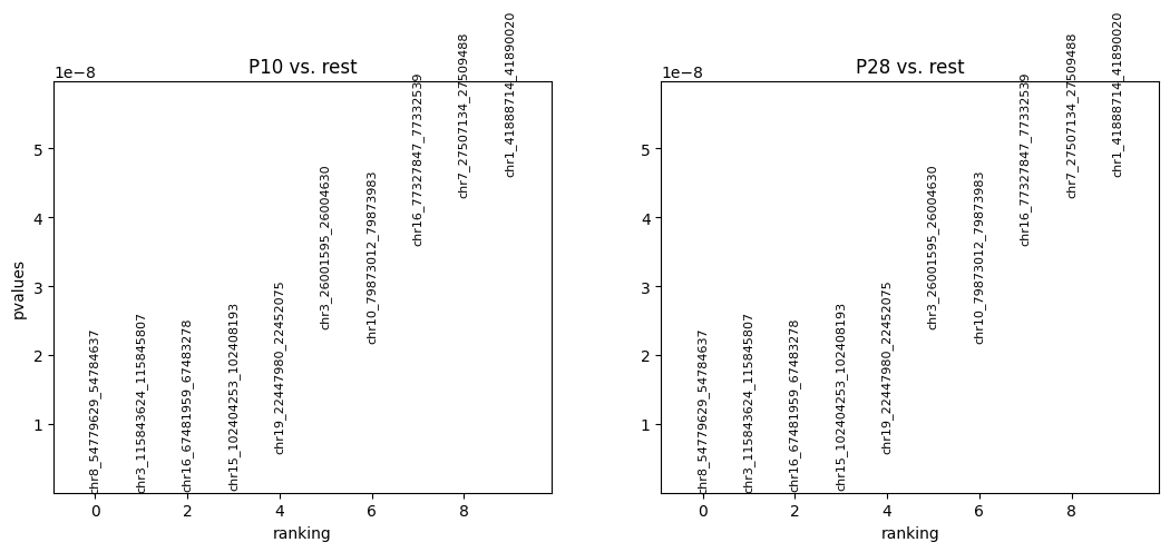
Plot the differential peak analysis results.
Currently, the peaks are ranked by pvalues. It could also be ranked by logfoldchanges by the following codes:
cc.tl.rank_peak_groups(adata_cc, 'Index', method = 'fisher_exact', key_added = 'fisher_exact',
                       rankby = 'logfoldchanges')
cc.pl.rank_peak_groups(adata_cc, key = 'fisher_exact', rankby = 'logfoldchanges')
[18]:
cc.pl.rank_peak_groups(adata_cc, key = 'fisher_exact')
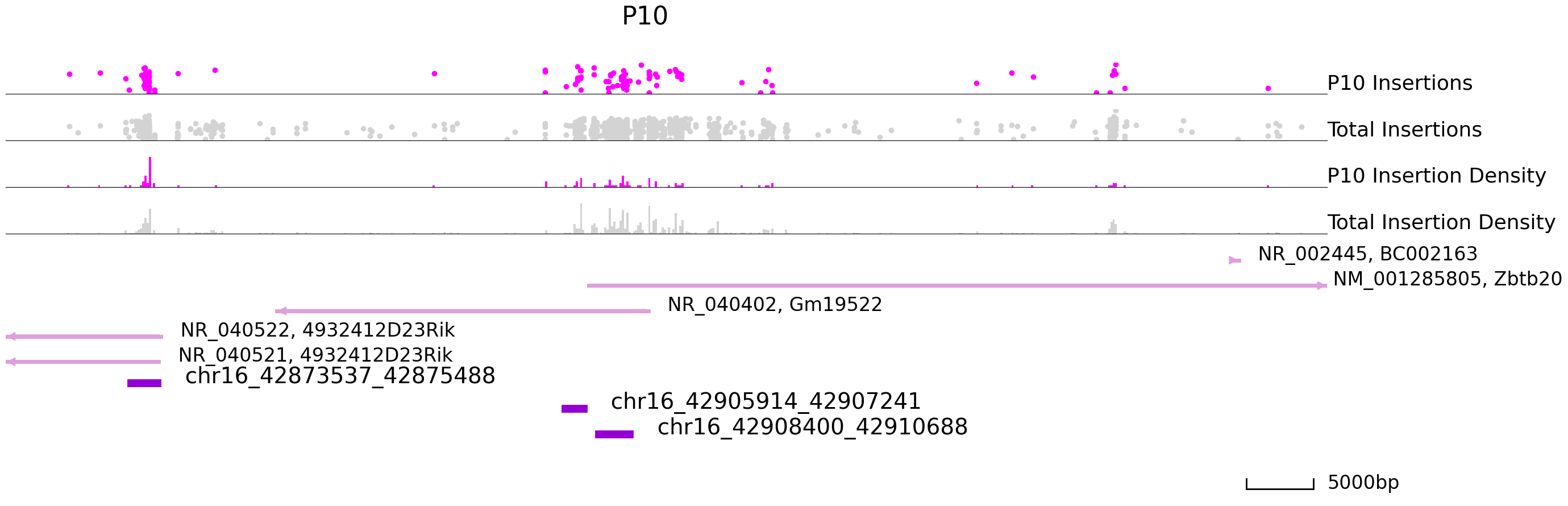
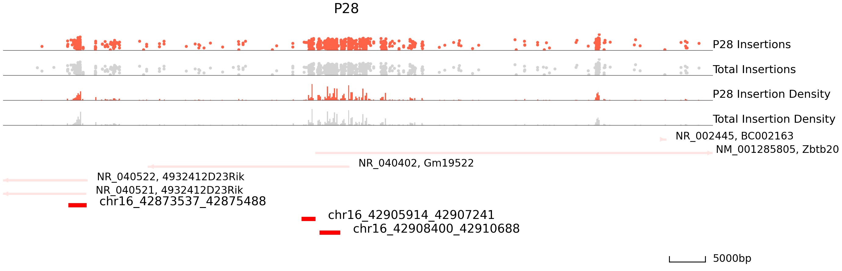
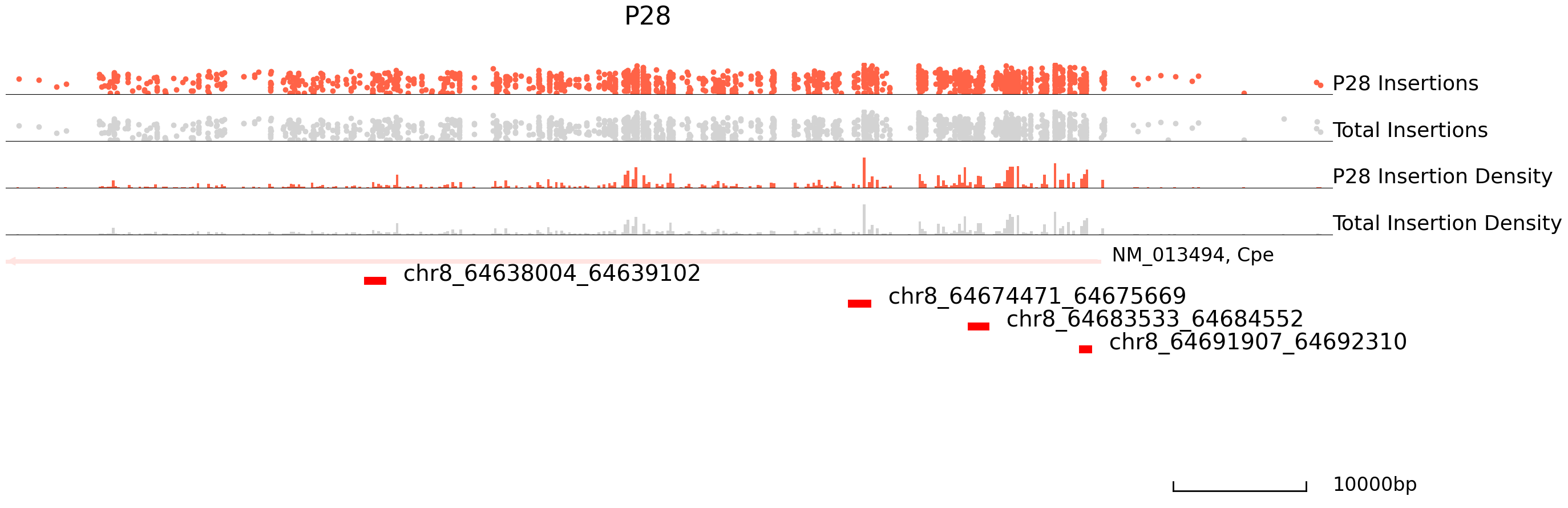
Next, we will visualize differentially bound peaks. The colored datapoints are the insertions specific to a cluster and the grey ones are the total insertions. If we input the backgound file, grey datapoints represent backgound insertions.
[19]:
cc.pl.draw_area("chr16", 42904181, 42922657, 40000, peak_data, SP1, "mm10", adata = adata_cc, font_size=2,
                name = "P10", key = "Index", insertionkey = "group", figsize = (30,10), plotsize = [1,1,4],
                name_insertion1 = 'P10 Insertions', name_density1 = 'P10 Insertion Density',
                name_insertion2 = 'Total Insertions', name_density2 = 'Total Insertion Density',
                peak_line = 3, bins = 600, example_length = 5000, color = "purple", title = "P10")
cc.pl.draw_area("chr16", 42904181, 42922657, 40000, peak_data, SP1, "mm10", adata = adata_cc, font_size=2,
                name = "P28",key = "Index", insertionkey = "group", figsize = (30,10), plotsize = [1,1,4],
                name_insertion1 = 'P28 Insertions', name_density1 = 'P28 Insertion Density',
                name_insertion2 = 'Total Insertions', name_density2 = 'Total Insertion Density',
                peak_line = 3, bins = 600, example_length = 5000, title = "P28")
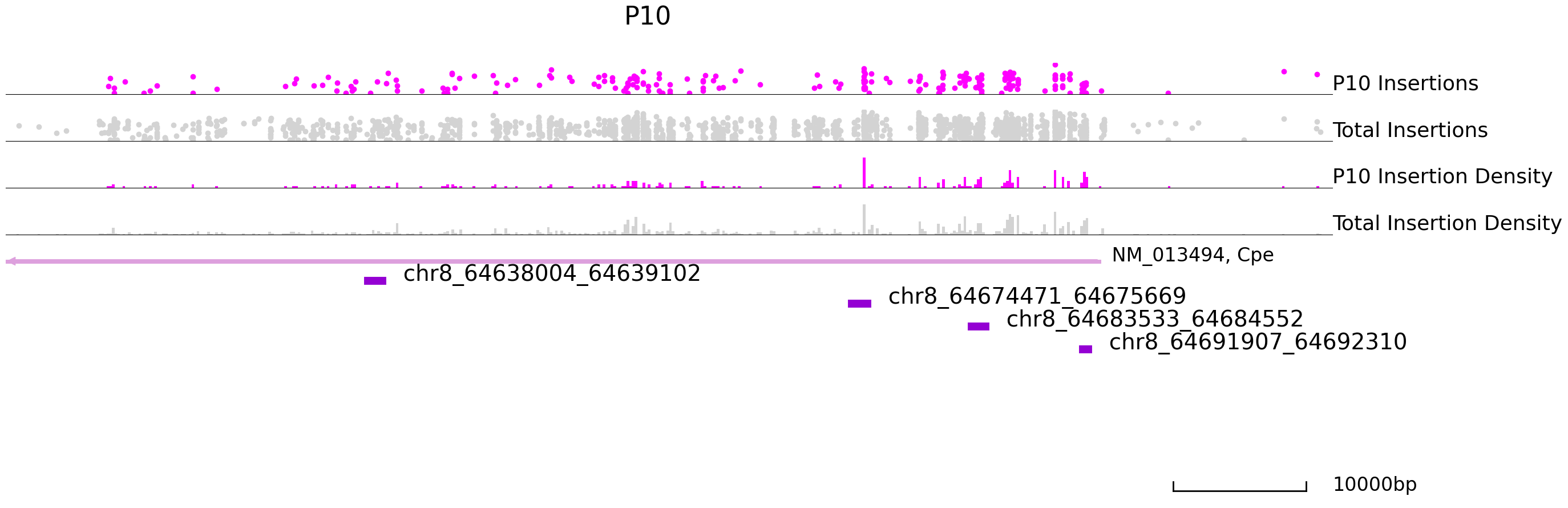
[20]:
cc.pl.draw_area("chr8", 64630703, 64690703, 20000, peak_data, SP1, "mm10", adata = adata_cc, font_size=2,
                name = "P10", key = "Index", insertionkey = "group", figsize = (30,10), plotsize = [1,1,4],
                name_insertion1 = 'P10 Insertions', name_density1 = 'P10 Insertion Density',
                name_insertion2 = 'Total Insertions', name_density2 = 'Total Insertion Density',
                bins = 500, peak_line = 8, color = "purple", title = "P10")
cc.pl.draw_area("chr8", 64630703, 64690703, 20000, peak_data, SP1,"mm10", adata = adata_cc, font_size=2,
                name = "P28", key = "Index", insertionkey = "group", figsize = (30,10), plotsize = [1,1,4],
                name_insertion1 = 'P28 Insertions', name_density1 = 'P28 Insertion Density',
                name_insertion2 = 'Total Insertions', name_density2 = 'Total Insertion Density',
                bins = 500, peak_line = 8, title = "P28")
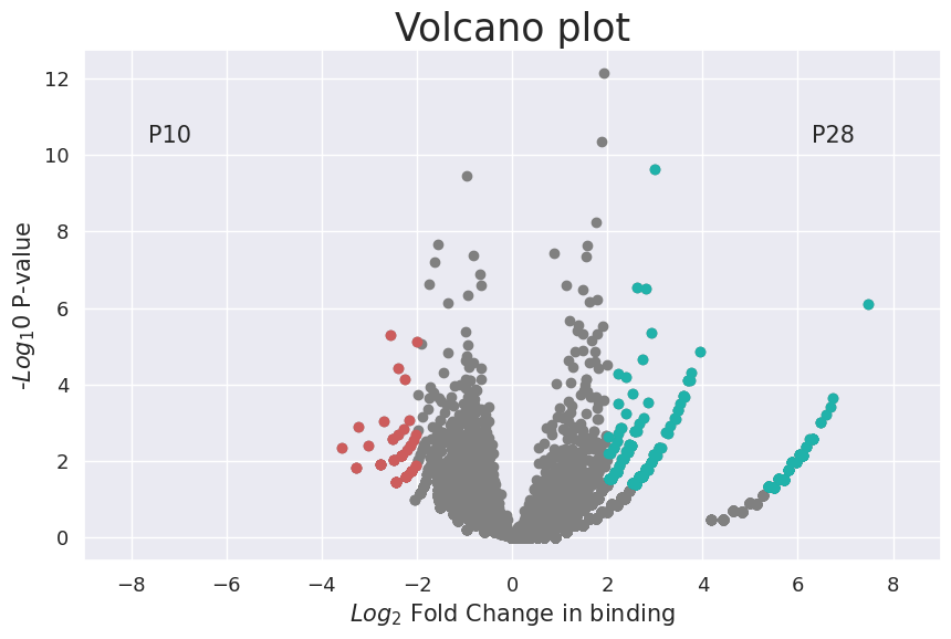
Plot the volcano plot for differential binding sites.
[21]:
cc.pl.volcano_plot(adata_cc, pvalue_cutoff = 0.05, lfc_cutoff = 2)
This is the heatmap for relative calling cards bindings.
[22]:
cc.pl.heatmap(adata_cc, figsize=(15,1))
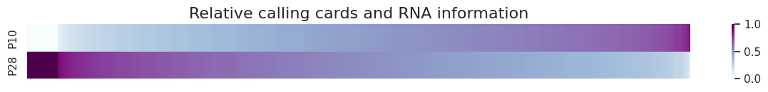
We can see from this plot that P28 has a considerable amount of additional Sp1 binding, as most peaks show increased binding at this timepoint. This is consistent with the experiment design as P28 is the accumulated insertions from day1 to day 28 while P10 reflect the insertions until day 10.
Save the file if needed.
[23]:
adata_cc.write("SP1_qbed.h5ad")